How to use RANDBETWEEN function in Excel

In this article, we will learn How to use the RANDBETWEEN function in Excel.

Scenario:

Random number generator means to get some random numbers between given numbers. Let's say if a user needs to get random numbers between 1-6 (roll of dice), the user doesn't need a dice for it. Excel provides you with function. Let's understand how function works and an example illustrates its use. You can also get random numbers in decimal.

RANDBETWEEN function in Excel

The RANDBETWEEN function in excel randomizes some numbers based on lower limit and upper limit.

RANDBETWEEN function Syntax

top : number cannot be above this number.

bottom : number cannot be lower than this number.

Note: RANDBETWEEN function is volatile and changes its value very soon. To record the numbers copy and paste only values.

Example :

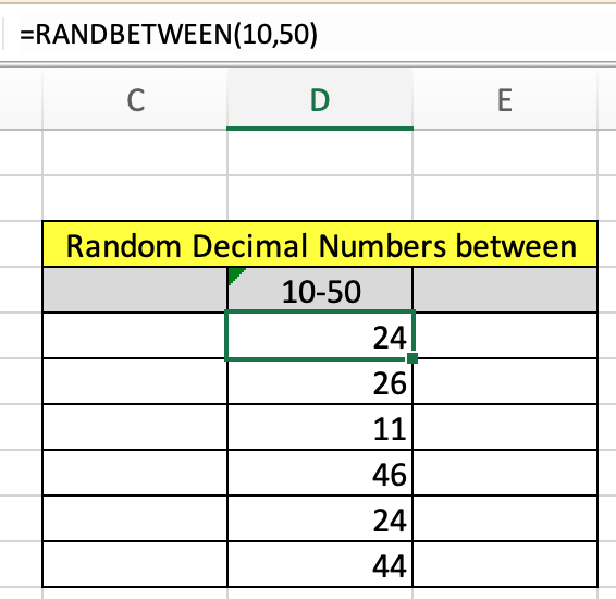
All of these might be confusing to understand. Let's understand how to use the function using an example. Here we have some examples to see how to get random numbers between 10 and 50.

Use the formula

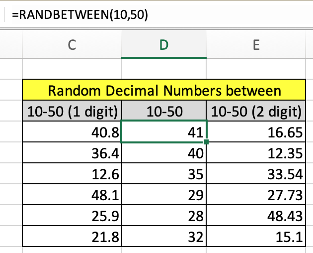
Just copy and paste this formula to the required number of times you need the result.Here only 6 numbers are generated. The RANDBETWEEN function only returns the whole number not any decimal number. But we can use it to convert the random decimal number.

Random decimal numbers with RANDBETWEEN function 

To get Random decimal numbers between two values let's say 1 to 10. So what can be the possible outcome 0.1, 1.234, 5.94, 3.5, 9.3222. It can be upto 1 decimal digit or 2 decimal digits. Now you don't need to worry. Let's say we have x and y two numbers. And we need to get 2 decimal digit numbers. So multiple both numbers with 100.

x -> 100x (new bottom number)

y -> 100y (new top number)

New formula

Let's get the random numbers between 10 and 50 upto 1 decimal digit.

Use the formula

As you can see now we decimal random numbers between 10 and 50. This simple method will solve the decimal number. Now similarly we can get the 2 decimal digit random numbers.

Use the formula

As you can clearly see random numbers between 2 numbers.

RANDOM TEXT values using RANDBETWEEN function

Now use the INDEX formula, this is more helpful than the CHOOSE formula as it doesn't require to input individual values. You can provide the fixed array using the naming the list using named range.

Use the formula :

list : named range used for A3:A14.

Explanation :

1. ROWS(table) returns the number of rows in the table which will be the last index of value in the list which is 12.
2. RANDBETWEEN function returns a random number from 1 to 12.
3. INDEX function will return the value corresponding to the returned number in the first column as list has only one column.

This is much simpler and easier. Now we will use the above formula for the value in the table.

RANDBETWEEN refreshes every time when something gets changed in the workbook. So when you are satisfied with the random data. Copy and paste values using the Paste special shortcut to get fixed values. You can learn how to get the random numbers or random date values in Excel

Here are all the observational notes using the formula in Excel
Notes :

1. The function refreshes every time when something changes in the workbook.
2. The RANDBETWEEN function returns an error, if the first number argument ( bottom ) is larger than the second number argument ( top ).
3. The RANDBETWEEN function returns error, if the argument to the function is non - numeric.
4. The function is mostly used to randomize a list in Excel or generate a random whole number.

Hope this article about How to use the RANDBETWEEN function in Excel is explanatory. Find more articles on generating values and related Excel formulas here. If you liked our blogs, share it with your friends on Facebook. And also you can follow us on Twitter and Facebook. We would love to hear from you, do let us know how we can improve, complement or innovate our work and make it better for you. Write to us at info@exceltip.com.

Related Articles :

Generate Random Phone Numbers : Generate random 10 digti numbers using the RANDBETWEEN formula in Excel.

Get Random number From Fixed Options : Generate random numbers form the list having criteria in Excel.

Get Random numbers between two numbers : RANDBETWEEN function generator number between the two given numbers in Excel.

Excel Random Selection: How to Get Random Sample From a Dataset : Use the random samples in Excel for the explained examples here.

How to use the RAND Function in Excel : Excel RAND function returns a number in Excel.

Relative and Absolute Reference in Excel : Understanding of Relative and Absolute Reference in Excel is very important to work effectively on Excel. Relative and Absolute referencing of cells and ranges.

Popular Articles :

How to use the IF Function in Excel : The IF statement in Excel checks the condition and returns a specific value if the condition is TRUE or returns another specific value if FALSE.

How to use the VLOOKUP Function in Excel : This is one of the most used and popular functions of excel that is used to lookup value from different ranges and sheets.

How to use the SUMIF Function in Excel : This is another dashboard essential function. This helps you sum up values on specific conditions.

How to use the COUNTIF Function in Excel : Count values with conditions using this amazing function. You don't need to filter your data to count specific values. Countif function is essential to prepare your dashboard.