So, we have already learned what 3D reference is in Excel. The fun fact is that the normal Excel 3D referencing does not work with conditional functions, like SUMIF function. In this article, we will learn how to get 3D referencing working with SUMIF function.
The generic formula for SUMIF with 3D reference in Excel
It looks complicated but it is not (that much).
| =SUMPRODUCT(SUMIF(INDIRECT("'"&name_range_of_sheet_names&"'!" & "criteria_range"),criteria,INDIRECT("'"&name_range_of_sheet_names&"'!" &"sum_range"))) |
"'"name_range_of_sheet_names"'": It is a named range that contains the sheet names. This is very important.
"criteria_range": It is the text reference of criteria containing range. ( It should be the same in all sheets to 3-D reference work.)
criteria: It is simply the condition that you want to put for summing. It can be a text or cell reference.
"sum_range": It is the text reference of the sum range. ( It should be the same in all sheets to 3-D reference work.)
Enough of the theory, let's 3D referencing with SUMIF function working.


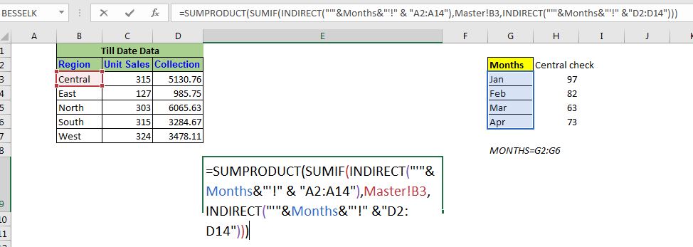
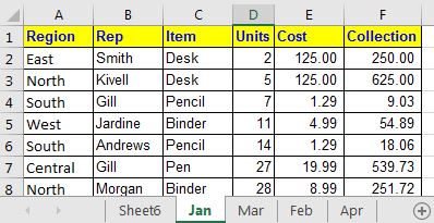
We are taking the same data that we took in the simple 3D referencing example. In this example, I have five different sheets that contain similar data. Each sheet contains a month's data. In the Master sheet, I want the sum of units and collection by region from all the sheets. Let's do it for Units first. The units are in the range D2:D14 in all the sheets.
Now if you use the normal 3D referencing with SUMIF function,
=SUMIF(Jan:Apr!A2:A14,Master!B4,Jan:Apr!D2:D14)
It will return #VALUE! error. So we can't use it. We will use the generic formula mentioned above.
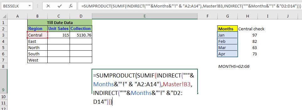
Using the above Generic 3D referencing SUMIF formula of excel, write this formula in cell C3:
| =SUMPRODUCT(SUMIF(INDIRECT("'"&Months&"'!" & "A2:A14"),Master!B3,INDIRECT("'"&Months&"'!" &"D2:D14"))) |
Here months is a named range that contains the names of sheets. This is crucial.
When you hit enter you get your exact output.
 How does it work?
The core of the formula is the INDIRECT function and the named range. Here the string "'"&Months&"'!" & "A2:A14" translates to an array of range references of each sheet in the named range.
| {"'Jan'!D2:D14";"'Feb'!D2:D14";"'Mar'!D2:D14";"'Apr'!D2:D14"} |
This array contains the text reference of ranges, not the actual ranges. Now since it is a text reference, it can be used by the INDIRECT function to convert them into actual ranges. This happens for both of the INDIRECT functions. After resolving the texts inside the INDIRECT functions (hold tight), the formula looks like this:
| =SUMPRODUCT(SUMIF(INDIRECT(({"'Jan'!A2:A14";"'Feb'!A2:A14";"'Mar'!A2:A14";"'Apr'!A2:A14"}), Master!B3,INDIRECT({"'Jan'!D2:D14";"'Feb'!D2:D14";"'Mar'!D2:D14";"'Apr'!D2:D14"}))) |
Now, the SUMIF function comes into action (not the INDIRECT, as you may have guessed). The condition is matched into the first range "'Jan'!A2:A14". Here the INDIRECT function works dynamically and converts this text into the actual range (that is why if you try to solve INDIRECT first using F9 key, you won't get the result). Next sums up the matched values in the range "'Jan'!D2:D14". This happens for each range in the array. Finally, we will have an array returned by the SUMIF function.
| =SUMPRODUCT({97;82;63;73}) |
Now the SUMPRODUCT does what it does best. It sums up these value and we get our 3D SUMIF function working.
So yeah guys, this how you can achieve a 3D SUMIF function. This is a bit complex, I agree on that. There's a lot of scope for errors in this 3D formula. I would suggest you use SUMIF function on each sheet in a definite cell and then use the normal 3D referencing for summing up those values.
I hope I was explanatory enough. If you have any doubts regarding excel referencing any other Excel/VBA related query, do ask in the comments section below.
Related Articles:
Relative and Absolute Reference in Excel | Referencing in excel is an important topic for every beginner. Even experienced excel users do mistakes in referencing.
Dynamic Worksheet Reference | Give reference sheets dynamically using the INDIRECT function of excel. This is simple...
Expanding References in Excel | The expanding reference expands when copied down or rightwards. We use the $ sign before the column and row number to do so. Here is one example...
All About Absolute Reference | The default reference type in excel is relative but if you want the reference of cells and ranges to be absolute use the $ sign. Here's all the aspects of absolute referencing in Excel.
Popular Articles:
50 Excel Shortcuts to Increase Your Productivity | Get faster at your task. These 50 shortcuts will make you work even faster on Excel.
The VLOOKUP Function in Excel | This is one of the most used and popular functions of excel that is used to lookup value from different ranges and sheets.
COUNTIF in Excel 2016 | Count values with conditions using this amazing function. You don't need filter your data to count specific value. Countif function is essential to prepare your dashboard.
How to Use SUMIF Function in Excel | This is another dashboard essential function. This helps you sum up values on specific conditions.
The applications/code on this site are distributed as is and without warranties or liability. In no event shall the owner of the copyrights, or the authors of the applications/code be liable for any loss of profit, any problems or any damage resulting from the use or evaluation of the applications/code.