Adding a Linked Picture to a Chart in Microsoft Excel 2010

In this article, we will learn about how we can move the chart to a different place in the sheet in Microsoft Excel 2010.

Before moving the chart to a different place in the sheet, we will learn how to create the chart.

Charts option contains 10 types of charts including Column, Line, Pie, Bar, Area, XY (Scatter), Stock, Surface, Radar, and Combo Charts.

We can create a chart by pressing the only one key on the keyboard.

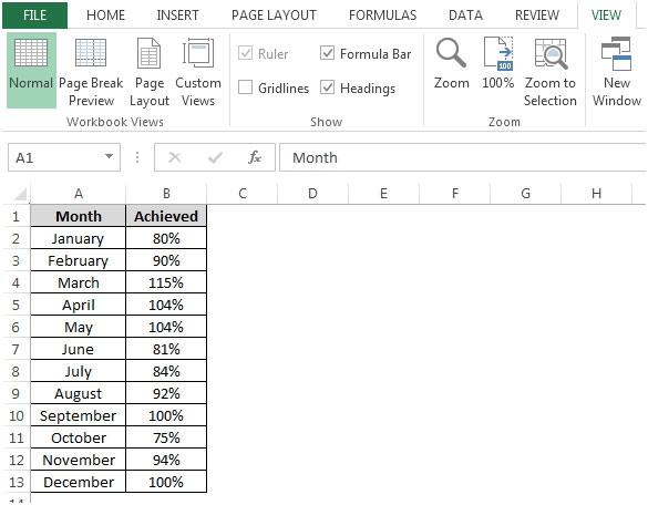
We have data in the range A1:B13. Column A contains Month, and Column B contains Achievement.
 

 
If we want to create a chart by using the F11 key, then we need to follow below given steps:-

• Select the cell A1 and press the key F11 on your keyboard.
• By default, column chart will get created in the new worksheet.

• In new worksheet, 2 contextual Tab Design and Format will appear in the main tab.
• By using the design tab, we can add the chart element, change the chart design, change the colors, switch Row/Column change the data range as well, and also we can move chart location as per the requirement.

• By using the format tab, we can insert the shapes, can change the shape style, color, we can insert the text in shapes, etc.

To move the chart to a different place in the sheet, follow below given steps:-

• We move the chart in Sheet1, then Go to design tab, and click on Move chart.
• Move Chart dialog box will appear.
• Click on object in, and then click on OK.

 
This is the way we can move the chart to a different place in the sheet in Microsoft Excel.

It would be an understatement to say that it is simple to update the text in an object.

For example, you add a title to the chart to indicate the period of the statement. A month later, the period of the financial statements changes, and you find yourself fighting to change the text in the object you have pasted into the chart.

When you link an object to a cell in the sheet, any change to the text in the cell will automatically update the text in the object.

Creating a picture of cells that is linked to the source data

In the sheet, copy a cell or cells that contain text or data, and paste it into the chart. Hold down Shift, and click Paste Picture Link on the Edit menu.

-OR-

Select a cell or cells, click the Camera icon, and then click where you want to paste the upper-left corner of the picture.

Adding the Camera icon to the toolbar:

Right-click any toolbar: From the shortcut menu, select Customize. Select the Commands tab, and from the Tools category, click and drag the Camera icon onto the toolbar.

Guidelines for working with linked pictures

Formatting – The linked text in the picture is formatted according to the formatting in the cell. Any changes to the formatting must be done in the source cell. You can change the formatting of the text; add text wrapping; change the width of a column or cell; omit gridlines (From the Tools menu, select Options, select the View tab, and then clear the Gridlines checkbox); and change the font color and cell shading (background color).

Note

Be sure to resize the column containing text you want in the picture before creating the link. Only the visible information in the cell will be included in the picture.

In the screenshot, two pictures have been pasted into a chart: a picture of the data table and a picture of the chart title.

The text, Sales Report for 3 years, was typed and formatted in a single cell in a different sheet. Screenshot // Adding a Linked Picture to a Chart in Microsoft Excel.