In this article, we will learn How to show details in the pivot table in Excel.
Scenario:
Problem pivot table is a powerful tool to summarize, analyse and visualize data. Pivot table group data based on given rows and columns fields. Now To drill down these grouped data we use the Show detail option in the Pivot table. For example if we need to see the branch wise distribution of employees. For situations like these we use a pivot table tool.
Show details pivot table in Excel
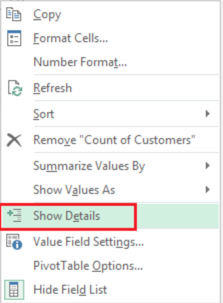
Select data > insert a new pivot table. Select any value in pivot table > Right click it > Select Show details.
Example :
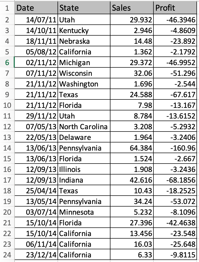
All of these might be confusing to understand. Let's understand how to use the function using an example. Here we have a sample data and its pivot table.
data

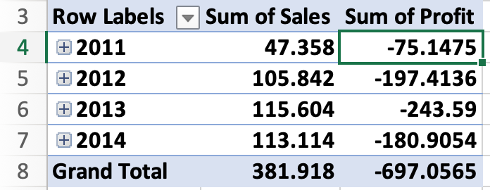
To insert Pivot table. Select data > Insert > Pivot table > Click Ok to get new pivot table in new sheet as shown below.
Pivot table

Now to view details of any cell value. Right any value from the sum of sales and profit columns.

Select Show details option as shown in the snapshot above. This option takes you to a new sheet with details of all the profit in 2011.

Show details option will elaborate the selected value in another sheet as shown above. This is the way to drill down a pivot table cell in excel. Learn more about pivot tables here.
Here are all the observational notes using the formula in Excel
Notes :
Hope this article about How to show details in the pivot table in Excel is explanatory. Find more articles on calculating values and related Excel tools here. If you liked our blogs, share it with your friends on Facebook. And also you can follow us on Twitter and Facebook. We would love to hear from you, do let us know how we can improve, complement or innovate our work and make it better for you. Write to us at info@exceltip.com.
Related Articles :
Excel Pivot Tables : Pivot tables are one of the most powerful tools and one who knows all the features of pivot tables can increase his productivity exponentially. In this article we will learn all about pivot tables in detail.
Conditional Formatting for Pivot Table : Conditional formatting in pivot tables is the same as the conditional formatting on normal data. But you need to be careful while conditional formatting pivot tables as the data changes dynamically.
How to get subtotal grouped by date using the GETPIVOTDATA function in Excel : This is a special function that is specially used to work with data from pivot tables. It is used to retrieve values from pivot tables using the table columns and rows headers.
How to use the Dynamic Pivot Table in Excel : To create a dynamic pivot table we use named ranges and tables in excel. But that is not all. A dynamic pivot table will reduce work of data maintenance and it will consider all newly added data as the source data.
How to Refresh Pivot Charts : To refresh a pivot table we have a simple button of refresh pivot table in the ribbon. Or you can right click on the pivot table. Here's how you do it.
Popular Articles :
How to use the IF Function in Excel : The IF statement in Excel checks the condition and returns a specific value if the condition is TRUE or returns another specific value if FALSE.
How to use the VLOOKUP Function in Excel : This is one of the most used and popular functions of excel that is used to lookup value from different ranges and sheets.
How to use the SUMIF Function in Excel : This is another dashboard essential function. This helps you sum up values on specific conditions.
How to use the COUNTIF Function in Excel : Count values with conditions using this amazing function. You don't need to filter your data to count specific values. Countif function is essential to prepare your dashboard.
The applications/code on this site are distributed as is and without warranties or liability. In no event shall the owner of the copyrights, or the authors of the applications/code be liable for any loss of profit, any problems or any damage resulting from the use or evaluation of the applications/code.
"Eric,
Make sure (if you have not done so already), that when you right click to bring up the grouping option, that you have the Date field highlighted first."
I have a pivot table with a date field that I want to group by quarter, month, year, etc. Everytime I click on group, I get an error box that says "Cannot group this section." Any ideas? Please advise. Thanks.
"Hi Gareth,
First question: Are the dates (you mention only months above) actually 'dates' as in date values in Excel, or are they text values (""Jan"",""Feb"") etc? Either way you should be able to filter to only show those you want using the pivot table filters that you seem to be applying already. You should not be getting those error messages.My first inclination is to try two things: 1) Try to do the same thing with a clean, small data set (perhaps copy and paste as values to a new workbook).Then re-create the pivot table with that clean small data set, and see what happens.If all is well, it would lead me to think that either your computer is low on memory, or the original data set is somehow corrupted and needs to be verified as a separate exercise (probably in Access?) 2) Re-install Excel. It could be that something in Excel that only gets used by pivot tables has been corrupted, and is causing those errors.If neither of those shed any light, post back and we can explore further.
Alan. "
"I am having some problems with the dates in my pivot tables, and I was hoping if someone new whether it is a limitation of Excel or not.I have various groupings, but it is pretty straightforward what I want to accomplish. I have a set of customers and I am trying to total Year To Date sales values i.e Year Month Account No. Customer Name Value Kilos 2003 Jan AAA123 Bob 100 20 ,Feb ABC234 Frank 250 20 ,etc However, I have 18 months worth of sales history in my Access database. Each customer purchases every month and there are around 10 customers in total in this particular scenario. I want my pivot table to allow me to define the range of months to display, i.e. Jan - Jul, but to total by customer for that period, and not show the month by month breakdown. The reason is that I want to try and build a comparison for the previous year, and this is where things go wrong. I get Dr. Watson application error messages appearing on my screen then excel gets killed Any one able to shine some light on the situation?
"