Currently, we can dynamically change or update pivot tables using Excel Tables or Dynamic Named Ranges. But these techniques are not foolproof. As you will still have to refresh the pivot table manually. If you have large data that contains thousands of rows and columns, excel tables will not help you a lot. Instead it will make your file heavy. So the only way remains is VBA.
In this article, we will learn how we can make our pivot table automatically change the data source. In other words, we will automate the manual process of changing data source to dynamically include new rows and columns added to source tables and reflect the change in pivot table instantly.
Since we want this to be completely automatic, we will use sheet modules to write code instead of a core module. This will allow us to use worksheet events.
If the source data and pivot tables are in different sheets, we will write the VBA code to change pivot table data source in the sheet object that contains the source data (not that contains pivot table).
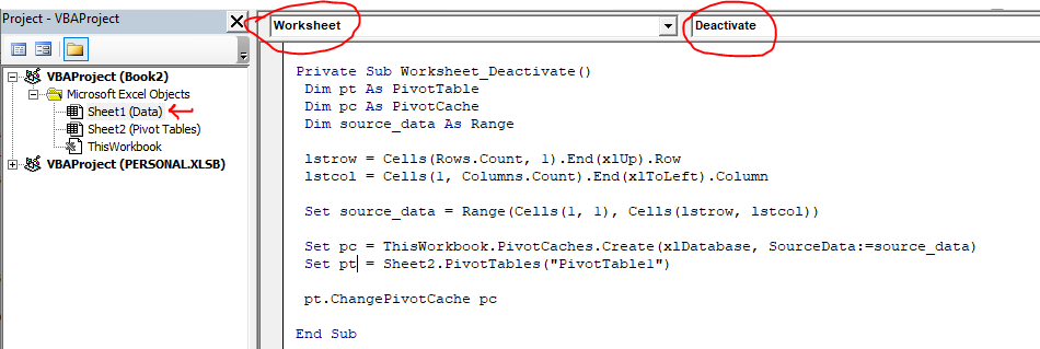
Press CTRL+F11 to open the VB editor. Now go to project explorer and find the sheet that contains the source data. Double click on it.

A new coding area will open. You may not see any change but now you have access to the worksheet events.
Click on the left drop down menu and select the worksheet. From the left drop down menu, select deactivate. You will see a blank sub written on the code area name worksheet_deativate. Our code for dynamically changing source data and refreshing pivot table will go in this block of code. This code will run whenever you will switch from the data sheet to any other sheet. You can read about all worksheet events here.

Now we are ready to implement the code.
To explain how it works, I have a workbook. This workbook contains two sheets. Sheet1 contains the source data that can change. Sheet2 contains the pivot table which depends on the source data of sheet2.
Now I have written this code in sheet1's coding area. I am using the Worksheet_Deactivate event, so that this code runs to update the pivot table whenever we switch from source data sheet.
Private Sub Worksheet_Deactivate()

 Dim pt As PivotTable

 Dim pc As PivotCache

 Dim source_data As Range


 lstrow = Cells(Rows.Count, 1).End(xlUp).Row

 lstcol = Cells(1, Columns.Count).End(xlToLeft).Column


 Set source_data = Range(Cells(1, 1), Cells(lstrow, lstcol))


 Set pc = ThisWorkbook.PivotCaches.Create(xlDatabase, SourceData:=source_data)

 Set pt = Sheet2.PivotTables("PivotTable1")


 pt.ChangePivotCache pc


End Sub
If you have a similar workbook, you can directly copy this data.I have explained this code works below.

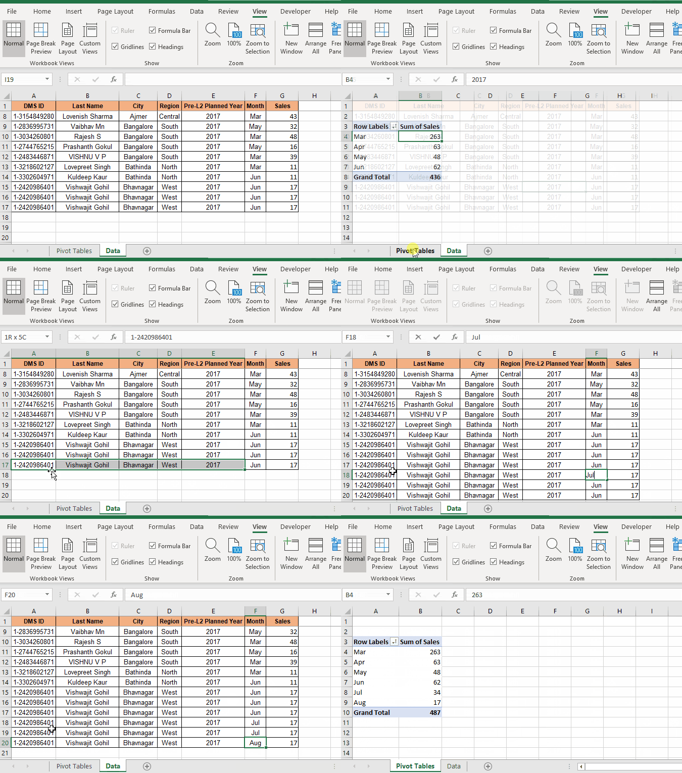
You can see the effect of this code in gif below.

How does this code automatically change source data and update pivot tables?
First of all we used a worksheet_deactivate event. This event triggers only when the sheet containing the code is switched or deactivated. So this is how the code automatically runs.
Now to change the source data of the pivot table we change data in the pivot cache.
A pivot table is created using pivot cache. The pivot cache contains the old source data until the pivot table is not manually refreshed or source data range is manually changed.
We have created references of pivot tables name pt, pivot cache named pc and a range named source_data. The source data will contain the whole data.
To dynamically get the whole table as data range we determine the last row and last column.
lstrow = Cells(Rows.Count, 1).End(xlUp).Row
lstcol = Cells(1, Columns.Count).End(xlToLeft).Column
Using these two numbers we define the source_data. We are definite that source data range will always start from A1.
Set source_data = Range(Cells(1, 1), Cells(lstrow, lstcol))
Now we have the source data which is dynamic. We just need to use it in the pivot table.
We store this data in pivot cache as we know pivot cache stores all the data.
Set pc = ThisWorkbook.PivotCaches.Create(xlDatabase, SourceData:=source_data)
Next we define the pivot table that we want to update. Since we want to update the PivotTable1 (name of pivot table. You can check the name of the pivot table in the analyze tab while selecting the pivot table.) on sheet1, we set pt as shown below.
Set pt = Sheet2.PivotTables("PivotTable1")
Now we simply use this pivot cache to update the pivot table. We use the changePivotCache method of pt object.
pt.ChangePivotCache pc
And we have our pivot table automated. This will automatically update your pivot table. If you have multiple tables with the same data source, just use the same cache in each pivot table object.
So yeah guys, this is how you can dynamically change data source range in Excel. I hope I was explanatory enough. If you have any questions regarding this article, let me know in the comments section below.
Related Articles:
How to Auto Refresh Pivot Tables Using VBA: To automatically refresh your pivot tables you can use VBA events. Use this simple line of code to update your pivot table automatically. You can use either of 3 methods of auto refreshing pivot tables.
Run Macro If Any Change Made on Sheet in Specified Range: In your VBA practices, you would get the need to run macros when a certain range or cell changes. In that case, to run macros when a change is made to a target range, we use the change event.
Run Macro When any Change is Made On Sheet | So to run your macro whenever the sheet updates, we use the Worksheet Events of VBA.
Simplest VBA Code to Highlight Current Row and Column Using | Use this small VBA snippet to highlight the current row and column of the sheet.
The Worksheet Events in Excel VBA | The worksheet event are really useful when you want your macros to run when a specified event occurs on the sheet.
Popular Articles:
50 Excel Shortcuts to Increase Your Productivity | Get faster at your task. These 50 shortcuts will make you work even faster on Excel.The VLOOKUP Function in Excel | This is one of the most used and popular functions of excel that is used to lookup value from different ranges and sheets.
COUNTIF in Excel 2016 | Count values with conditions using this amazing function. You don't need filter your data to count specific value. Countif function is essential to prepare your dashboard.
How to Use SUMIF Function in Excel | This is another dashboard essential function. This helps you sum up values on specific conditions.
The applications/code on this site are distributed as is and without warranties or liability. In no event shall the owner of the copyrights, or the authors of the applications/code be liable for any loss of profit, any problems or any damage resulting from the use or evaluation of the applications/code.