How to Format a PivotTable Report in Excel

In this article, we will learn How to Format a PivotTable Report in Excel.

Scenario:

In excel, everyone uses a pivot table to summarize, analyze and visualize data in grouped format. But few want to change the pivot table color, size, font. Rest all of us use the default pivot table style. So if you are frustrated using the same default style every time then you have arrived at the right place after wandering for a long time. Let's learn where to find the pivot table styles and how to use it explained here illustrating an example.

Pivot table formatting in Excel

First we need to make a pivot table in excel

Select data > insert a new pivot table.

Change Pivot table layout

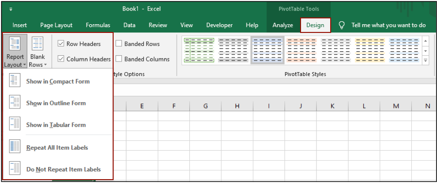
Select any value in pivot table > Go to Design > Report Layout > then select from the options shown below.

Show in Compact Form
Show in Outline Form
Show in Tabular Form

Change Pivot table layout

Select any value in pivot table > Go to Design > Select any style from the pivot table styles

Example :

All of these might be confusing to understand. Let's understand how to use the function using an example. Here we have data. First we need to insert a new pivot table for the format.

To insert Pivot table. Select the data > Insert > Pivot table > Click Ok to get new pivot table in new sheet as shown below.

You can view the pivot table in the new sheet. It will be something like shown below.

Now to change its default view. Select any pivot table cell and as you can see, as soon as you select any cell from the pivot table. Two new tabs displayed above. Go to Design tab > Report Layout. The same can be viewed from below snapshot

Excel shows you four options. Select any to apply the required layout. Now to change its Format view. Select any pivot table cell and as you can see, as soon as you select any cell from the pivot table. Two new tabs displayed above. Go to the Design tab > Pivottable Styles. The same can be viewed from the below snapshot.

There are so many recommended styles but you can create your own using the New pivot table style. Select the type of style and say no to default pivot style in excel.

Here are all the observational notes using the formula in Excel
Notes :

Create new pivot table columns using pivot table fields option under the analyze tab of pivot table ribbon in excel.
Sort the data after filtering which makes it easier to read.
You can create a pivot table on the same sheet as data or in a different sheet of the same workbook.
Use the recommended pivot table for quick and advanced summarization.

Hope this article about How to Format a PivotTable Report in Excel is explanatory. Find more articles on calculating values and related Excel formulas here. If you liked our blogs, share it with your friends on Facebook. And also you can follow us on Twitter and Facebook. We would love to hear from you, do let us know how we can improve, complement or innovate our work and make it better for you. Write to us at info@exceltip.com.

Related Articles :

Excel Pivot Tables : Pivot tables are one of the most powerful tools and one who knows all the features of pivot tables can increase his productivity exponentially. In this article we will learn all about pivot tables in detail.

Conditional Formatting for Pivot Table : Conditional formatting in pivot tables is the same as the conditional formatting on normal data. But you need to be careful while conditional formatting pivot tables as the data changes dynamically.

How to get subtotal grouped by date using the GETPIVOTDATA function in Excel : This is a special function that is specially used to work with data from pivot tables. It is used to retrieve values from pivot tables using the table columns and rows headers.

How to use the Dynamic Pivot Table in Excel : To create a dynamic pivot table we use named ranges and tables in excel. But that is not all. A dynamic pivot table will reduce work of data maintenance and it will consider all newly added data as the source data.

How to Refresh Pivot Charts : To refresh a pivot table we have a simple button of refresh pivot table in the ribbon. Or you can right click on the pivot table. Here's how you do it.

Popular Articles :

50 Excel Shortcuts to Increase Your Productivity : Get faster at your tasks in Excel. These shortcuts will help you increase your work efficiency in Excel.

How to use the VLOOKUP Function in Excel : This is one of the most used and popular functions of excel that is used to lookup value from different ranges and sheets.

How to use the IF Function in Excel : The IF statement in Excel checks the condition and returns a specific value if the condition is TRUE or returns another specific value if FALSE.

How to use the SUMIF Function in Excel : This is another dashboard essential function. This helps you sum up values on specific conditions.

How to use the COUNTIF Function in Excel : Count values with conditions using this amazing function. You don't need to filter your data to count specific values. Countif function is essential to prepare your dashboard.