Insert Calculated Field in Pivot Table in Microsoft Excel 2010
In this article we will lear how to we can add a data field that calculates the difference between two data fields in Mcirosoft Excel 2010.
“PIVOT TABLE”is used for Summarize alarge amount number of data without using any formulas, it makes the data easy to read with flexibility.
Let’s take an example to add data fields that calculate the difference between two data fields.
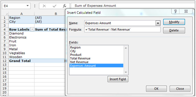
I have a “PIVOT TABLE” in which Column A containsthe product column B sum of total revenue in column C net revenue. We need to show the expenses amount inthe “PIVOT TABLE”. We need to follow the below mentioned steps to add the data field in the “PIVOT TABLE”.:-

- Click on any cell in the pivot table report, the contextual menu on the ribbon will get activated.
- Go to the “Analyze” tab, in the “Calculations” group select “Calculated Field” from the “Field, Items & Sets” drop down list.
- The dialog box will appear, type “Expenses Amount”as the name ofthe new field in the “Name” box.

- In the “Fields” box select “Total Revenue” and click on the “Insert Field” button or double click on “Total Revenue” directly to insert it in the Formula box. Type the minus (-) sign in the “Formula” box.
- Select “Net Revenue” from the “Field” box and click on “Insert Field” or double click as mentioned above.
- Click on ok.
The field will appear as another column in the pivot table.

Now let’saddanother data field in the “PIVOT TABLE” -
- Click on any cell in the pivot table report, the contextual menu on the ribbon will get activated.
- Go to the “Analyze” tab, in the “Calculations” group select “Calculated Field” from the “Field, Items & Sets” drop down list.
- The dialog box will appear, type “%age of Expenses” as the name of the new field in the “Name” box.
- In the “Field” box select “Expenses Amount” and click on “Insert Field” or double click on Expenses Amount,type division (/) sign in the “Formula” box.
- Select “Total Revenue” from “Field” box and click on “Insert Field” or double click on Total Revenue.

- Click on ok.
- To change the field to %age format, select the range E5:E12, and press the key “CTRL+SHIFT+ %( 5)”.
- The Range will be formatted as a %age.


Hi, I did what you've done and my results showing as millions but my numbers is as simple as 209 - 361 and then division is 0
can you advise what I've done wrong.