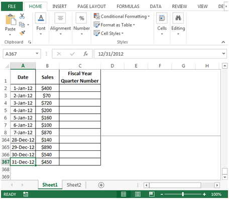
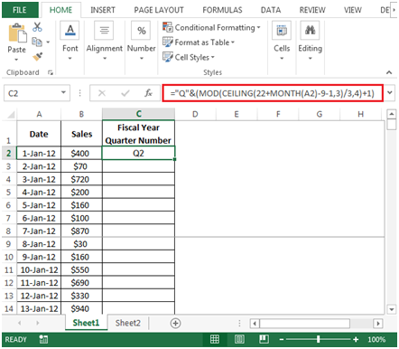
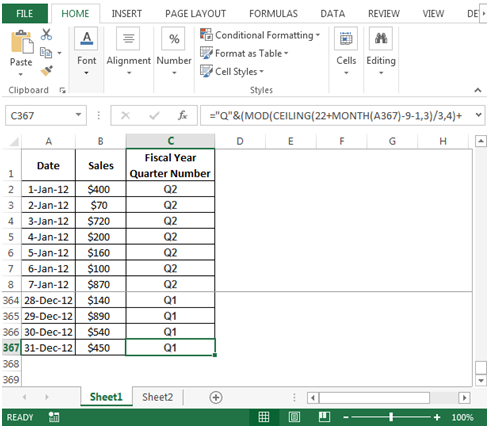
Pivot Table Report Grouping Date Field in Microsoft Excel 2010

To make use of grouping the date field by quarter in pivot table report, we can use a combination of MOD, CEILING & MONTH functions to get the output.

Let us take an example:

Column A contains Dates & column B contains Sales.We need a formula to calculate the Quarter number in a Fiscal year. For example, Q1 will start from 1-Oct to 31-Dec, Q2 from 1-Jan to 31-Mar, Q3 from 1-Apr to 30-Jun, Q4 from 1-Jul to 30-Sep.

In cell C2, the formula would be
="Q"&(MOD(CEILING(22+MONTH(A2)-9-1,3)/3,4)+1)

Copying down the formula in below shown range, we will get the desired result.

To make use of Quarters in a Fiscal year, we need to create a pivot table report.

Arrange the fields as shown in below shown snapshot.

To view the entire report quarter wise, you need to click on any cell in column A & right click
Select Expand/Collapse & then click on Collapse Entire Field

You will be able to view the report quarter wise.

In this way we can group in excel.

Jody Bennett
December 11, 2014 at 3:32 pm

I commonly refer to Quarters in my pivot tables but I use the CHOOSE function. The formula looks like this.
=CHOOSE(MONTH(A2),1,1,1,2,2,2,3,3,3,4,4,4)
Great post, I love this site!

Reply ↓

Leave a Reply Cancel reply

Terms and Conditions of use

The applications/code on this site are distributed as is and without warranties or liability. In no event shall the owner of the copyrights, or the authors of the applications/code be liable for any loss of profit, any problems or any damage resulting from the use or evaluation of the applications/code.