PivotTable report - Grouping the Date Field by Week Number in Excel 2010

In a pivot table, in order to group the dates, number and text fields or group dates by year and month. We can manually select the items in a pivot table field, and group the selected items. This will help us in findingthe subtotals for a specific set of items in the pivot table.

To create a pivot table report – grouping the date field by week, let us first create a pivot table report.
Let us take an example:

• We have dates in column A from 1-Jan-2012 to 31-Mar-2013

• Click on Insert Ribbon to create a pivot table report
• In Tables group, click on Pivot Table

• Create Pivot Table dialog box will appear

• Select existing worksheet option if we want to create the report in existing worksheet, otherwise click on OK to create the table in a new worksheet.

• Drag Date to Rows field & Sales to Values field.

• Now we need to click on any cell in column A (Date column) & right click and select Group option

• Select Days& enter 7 in number of days as shown below in snapshot

• Click on OK, and we will see the Sales will be segregated week wise.

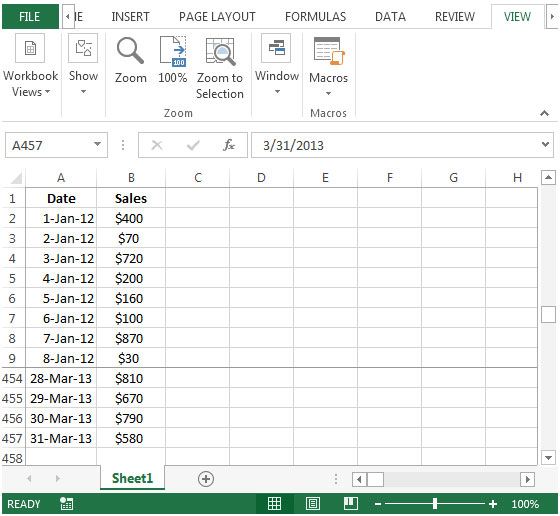
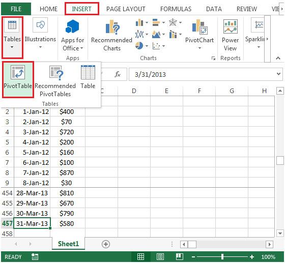
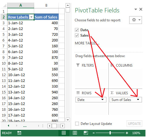
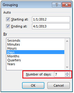
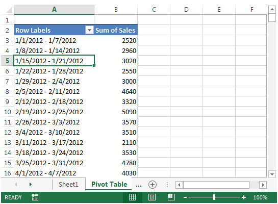
Grouping the dates will allow us to quickly find the sales in a particular period.