In this article, we will learn how to show hide Field Header in pivot table in Excel 2016.
For that first, we need to understand how the pivot table works in excel 2016.
A pivot table allows you to extract the data from a large, detailed data set into a customized data set.
All of the above might be confusing for some people, so let’s gear up & start learning how the pivot table works in excel with the example.
Shown below is a data set.
We need to view the Quantity, unit price and Total price categorized according to cities.
We just need to select the data and create its pivot table in just a few simple steps.
Create Pivot table dialog box appears
Select the Table/Range and choose New worksheet for your new table and click OK.
Your new worksheet will be here like shown below
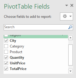
Now you need to select the fields from the pivot table fields on the right of your sheet.
Now we need Quantity, unit price and Total price categorized according to cities.

Select the required fields to get the pivot table as shown below.

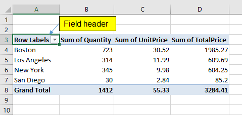
Finally, my data is sorted in a way I wanted.
But I don’t require the field header. To remove the field header. Select Analyze > then unselect field header

You will see that the field header has been removed.

You can create and customize your table with the Pivot table function in Excel.
Hope you understood how to remove field header from the pivot table in Excel 2016. Find more articles on pivot table here. Please share your query below in the comment box. We will assist you.
Popular Articles:
50 Excel Shortcuts to Increase Your Productivity
How to use the VLOOKUP Function in Excel
The applications/code on this site are distributed as is and without warranties or liability. In no event shall the owner of the copyrights, or the authors of the applications/code be liable for any loss of profit, any problems or any damage resulting from the use or evaluation of the applications/code.