In this article, we will learn The Pivot table tools ribbon in Excel.
Scenario:
Pivot table is the most popular tool to calculate, analyse and summarize the whole data. But here the problem is to extract top 10 or bottom 10 items. For example getting the top 10 salespeople who sold the most products or getting to know the bottom 10 salespeople who sold the least products in a company. Or it could be finding the top 10 customers who bought the most products. For these kinds of problems we use a pivot table and its row label fields.
The PivotTable Tools Ribbon contains two tabs:
First Create a pivot table
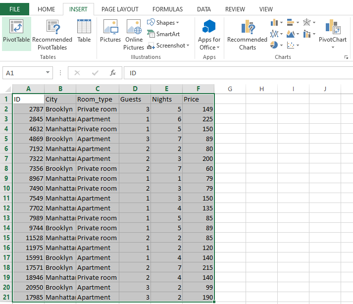
Select the data with labels (column names) > Insert tab > Pivot table > Select same worksheet or new worksheet > Click OK.
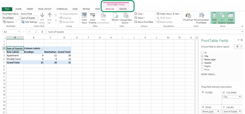
Now use column names to add values to the pivot table. On the menu bar you can see Pivot table tools which are marked under different colour.
Example :
All of these might be confusing to understand. Let's understand how to use the function using an example. Here we have data and we need to access the pivot table ribbon for the data. Follow the steps.
Create a pivot table for the data. Select the data and Go to Insert tab and select pivot table option as shown below.

Select the required options and click Ok and you will have the pivot table and pivot table fields as shown below.

On the right hand side. Choose the fields to start using a pivot table. As you can see when you select any pivot table cell and some tabs glows on the top named Pivot table tools.

These two tabs allow you to perform pivot table customization. This is the Pivot table ribbon in Excel. Create pivot table fields , charts and sets.
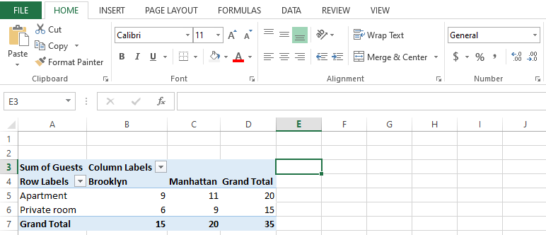
Here is an important thing to wonder for the pivot table ribbon in excel is as soon as you switch the selected cell to non pivot table cell. The pivot table ribbon disappears. So it means Excel only allows you to use pivot table options when you select the pivot table cell as shown below.

Now as you can see the pivot table ribbon disappears. That's the common problem excel users face. Hope it won't be an issue after now.
Here are all the observational notes using the formula in Excel
Notes :
Hope this article about The Pivot table tools ribbon in Excel is explanatory. Find more articles on calculating values and related Excel formulas here. If you liked our blogs, share it with your friends on Facebook. And also you can follow us on Twitter and Facebook. We would love to hear from you, do let us know how we can improve, complement or innovate our work and make it better for you. Write to us at info@exceltip.com.
Related Articles :
Excel Pivot Tables : Pivot tables are one of the most powerful tools and one who knows all the features of pivot tables can increase his productivity exponentially. In this article we will learn all about pivot tables in detail.
Conditional Formatting for Pivot Table : Conditional formatting in pivot tables is the same as the conditional formatting on normal data. But you need to be careful while conditional formatting pivot tables as the data changes dynamically.
How to get subtotal grouped by date using the GETPIVOTDATA function in Excel : This is a special function that is specially used to work with data from pivot tables. It is used to retrieve values from pivot tables using the table columns and rows headers.
How to use the Dynamic Pivot Table in Excel : To create a dynamic pivot table we use named ranges and tables in excel. But that is not all. A dynamic pivot table will reduce work of data maintenance and it will consider all newly added data as the source data.
How to Refresh Pivot Charts : To refresh a pivot table we have a simple button of refresh pivot table in the ribbon. Or you can right click on the pivot table. Here's how you do it.
Popular Articles :
50 Excel Shortcuts to Increase Your Productivity : Get faster at your tasks in Excel. These shortcuts will help you increase your work efficiency in Excel.
How to use the VLOOKUP Function in Excel : This is one of the most used and popular functions of excel that is used to lookup value from different ranges and sheets.
How to use the IF Function in Excel : The IF statement in Excel checks the condition and returns a specific value if the condition is TRUE or returns another specific value if FALSE.
How to use the SUMIF Function in Excel : This is another dashboard essential function. This helps you sum up values on specific conditions.
How to use the COUNTIF Function in Excel : Count values with conditions using this amazing function. You don't need to filter your data to count specific values. Countif function is essential to prepare your dashboard.
The applications/code on this site are distributed as is and without warranties or liability. In no event shall the owner of the copyrights, or the authors of the applications/code be liable for any loss of profit, any problems or any damage resulting from the use or evaluation of the applications/code.