While working on Excel, you must have heard about named ranges in excel. Maybe from a friend, colleague or some online tutorial. Even I have mentioned it many times in my articles. In this article, we will learn about the Named Ranges in Excel and will explore every aspect of it.
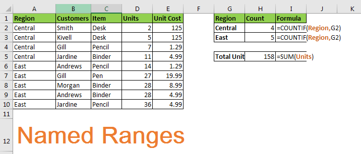
Well, named ranges are nothing but some excel ranges that a tagged with some meaningful name. For example, if you have a cell say B1, contains the everyday target, you can name that cell as specifically “Target”. Now you can use “Target” to refer at A1 instead of writing B1.
In a nutshell, Named range is just naming of ranges.
To define a name to a range, you can use shortcut CTRL+F3. Or you can follow these steps.

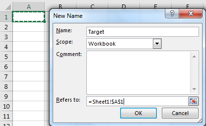
Now you can refer to it by just typing its name.
There are some rules to follow while creating names. They are
Well, most of the time you will be working with a structured data table. They will have column and rows with column headings and row headings. And most of the time these names are meaningful to the data, and you’d like to name your range as these column headings. Excel provides a tool to name ranges using titles automatically. Follow these steps.
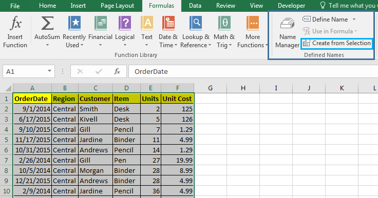
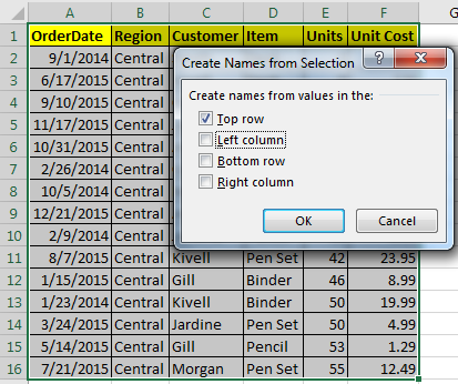
Now each column is named as their heading. Whenever you typewill type a formula, these name will be listed in option to be used.
When we organise a data as a table in excel using CTRL + T, the column headings are automatically assigned as the name of the respective column. You should explore Excel Tables and their benefits.
Well, there will be times when you would like to see all available named ranges in the workbook. To see all name ranges Press CTRL+F3. Or you can go to Formula Tab > Name Manager. It will list all named ranges that are available on the workbook. You can Edit available named ranges, delete them, add new names.
Excel allows users to name the same range with different names. For example range A2:A10 can be named ‘Customers’ and ‘Clients’ both at the same time. Both names will refer to the same range A2:A10.
But you can’t have the same names for two different ranges. It eliminates the chance of ambiguity.
So if you want to have a list of named ranges and the ranges they are covering you can use this shortcut for pasting them on a place in a sheet.


If you double click on the named ranges name in the paste name box, they will get written as formulas in the cell. Try it.
Well, when you insert a cell inside a named range, it updates automatically and expands it. But if you add data at the end of the table, you’ll need to update the named field. To update Named Ranges, follow these steps.
And It's done. This is manual updating of named ranges. However, we can make it dynamic by using some formulas.
It is wise to make your named ranges dynamic so that you don’t have to edit them whenever your data overflows the predefined range.
I have covered it in a separate article called Dynamic Named ranges. You can learn and understand the benefits of it in detail here.
When you delete some part of named range, it auto-adjusts its range. But when you delete whole name range the vanishes from the name list. Any formula, dependent on those ranges will show #REF error, or they will give incorrect output (counting functions).
For any reason, if you want to delete named ranges, follow these steps.
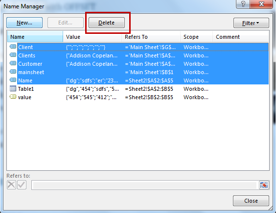
Caution: Before you delete the named ranges, make sure that no formulas are dependent on these names. If there is any, convert them to ranges first. Otherwise you’ll see #REF error.
Excel provides a tool to remove names that have errors only. You don’t need to identify each of them by yourself. To delete names with errors, follow these steps:

And they are gone. All the names with errors will be deleted from record immediately.
Best use of named ranges is experienced with formulas. The formulas get more flexible and readable with Named Ranges. Let’s see how.
Now let’s say you have named a range as “Items”. Now the Items list you want to count “Pencils”. With name, it is easy to write this COUNTIF formula. Just write
=COUNTIF(Item, "Pencil")
As soon as you write the opening parenthesis of formula, the list of available named ranges will appear. Without a name you would write a gi COUNTIF function of Excel with ranges, for which you may have to look at the range first then select the range or type it in the formula.
The names of ranges are shown as suggestions when you type any letter after = sign. Same as excel shows the list of formulas. For example, if you type =u, each method and named range will be displayed starting with u, so that you can use them easily.

So far, we learned about naming ranges, but you can actually name values too. For example, if your client name is Sunder Pichai than you can make a name “Client” and it refers to write “Sundar Pichai”. Now, whenever you write =Client in any cell, it will show Sundar Pichai.

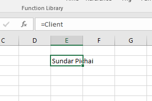
Not only text, but you can also assign a number as constant to work with. For example, you define a target. Or the value of something that will not change.
Absolute and Relative Referencing with Named Ranges
The referencing with Named ranges in is very flexible. For example, if you write the name of a named range in relative cell, it will behave like a corresponding reference. See below image.
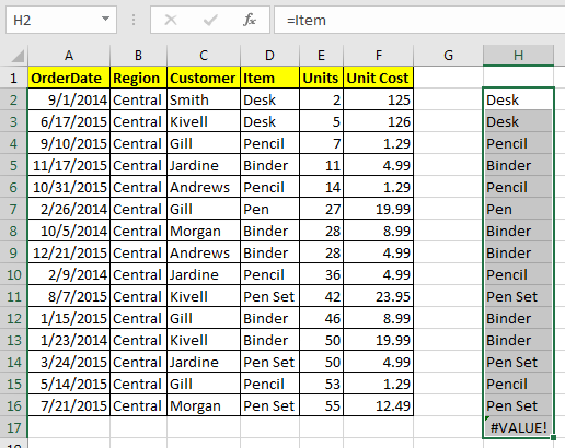
But when you use it with formulas, it will behave as absolute. Well, most of the time you’ll be using them with formulas, so you can say that they are by default Absolute, but actually they are flexible.
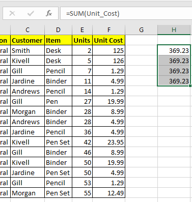
But we can make them relative too.
Let’s say if I want to name a range “Before” which will refer to cell left to wherever it is written. How do I do that? Follow these steps:

Now wherever you will write “Befor” in formula, it will refer to cell left to it.

Here, I used before in COLUMN function. The formula returns the column number of the left cell where it is written. To my suprise, A1 shows the column number of last column. Which means the sheet is circulare. I thought it will show an #REF error.
Now this one is amazing. Many times you use same formula again and again in a worksheet. For example you may want to check if a name is in your customer list or not. And this need may occur many times. For this you’ll write same complex formula every time.
How about, if you just type ‘=IsInCustomer’ in a cell and it will show you if the value in left cell is in customer list or not?
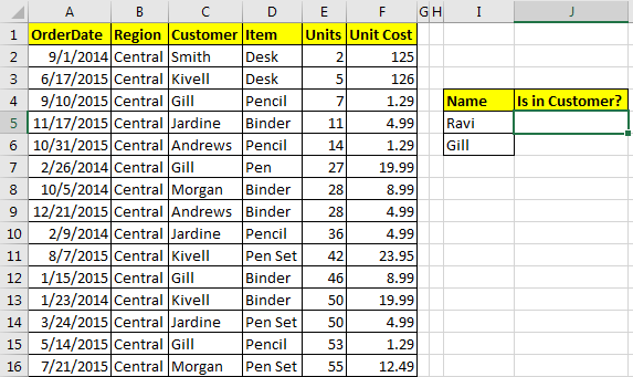
For example, I have prepared a table here. Now i just want to type “=IsInCustomer” in J5 and i would like to see if the value in I5 is in Customer list or Not. To do so follow these steps.

Now wherever you type ‘IsInCustomer’, It will check the value in left cell in Customer list.

This stop you from repeating your self again and again.
So many times, we define names to our ranges after we have already written formulas based on ranges. For example I have Total Price as Cells =E2*F2. How can we change it to Units*Unit_Cost.
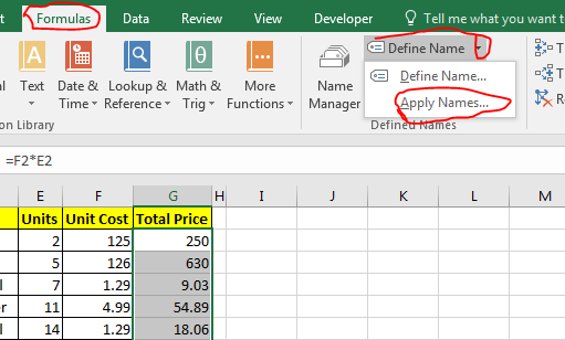
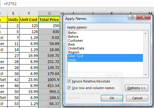
And the names are now applied. You can see it in formula bar.

As you’ve seen that named ranges make it easy to read the formulas. If I write =COUNTIF(“A2:A100”,B2), no one will understand what I am trying to count, until they see the data or someone explains it to them.
But if I write =COUNTIF(region,’east’), most users will immediately get it that we are counting occurrence of ‘east’ in region named range.
Named ranges make it very easy to copy and paste formulas without worrying about changing references. And you can take one formula from one workbook to another and it will work fine until and unless destination workbook have same names.
Fore example if you have a Formula =COUNTIF(region,east) in Distribution Table and you have another workbook say customers that also has a named range “Region”. Now if you copy this formula directly anywhere on that workbook it will show you correct information. The structure of data will not matter. It doesn’t matter where the hell is that column in your workbook. This will work correctly.

In the above image I have used exact same formula in two different file to count number or east occuring in region list. Now they are in different columns but since both of then are named as region it will work perfectly.
It gets easier to navigating in workbook with named ranges. You just need to type name of the named in name box. Excel will take you to the range, doesn’t matter where are you in the workbook. Given that named range is of Workbook scope.
For example, if you are on sheet10 and you want want to got customer list, and you don’t know on which sheet it is. Just go to name box and type ‘customer’. You’ll be directed to the named range in fraction of a second.
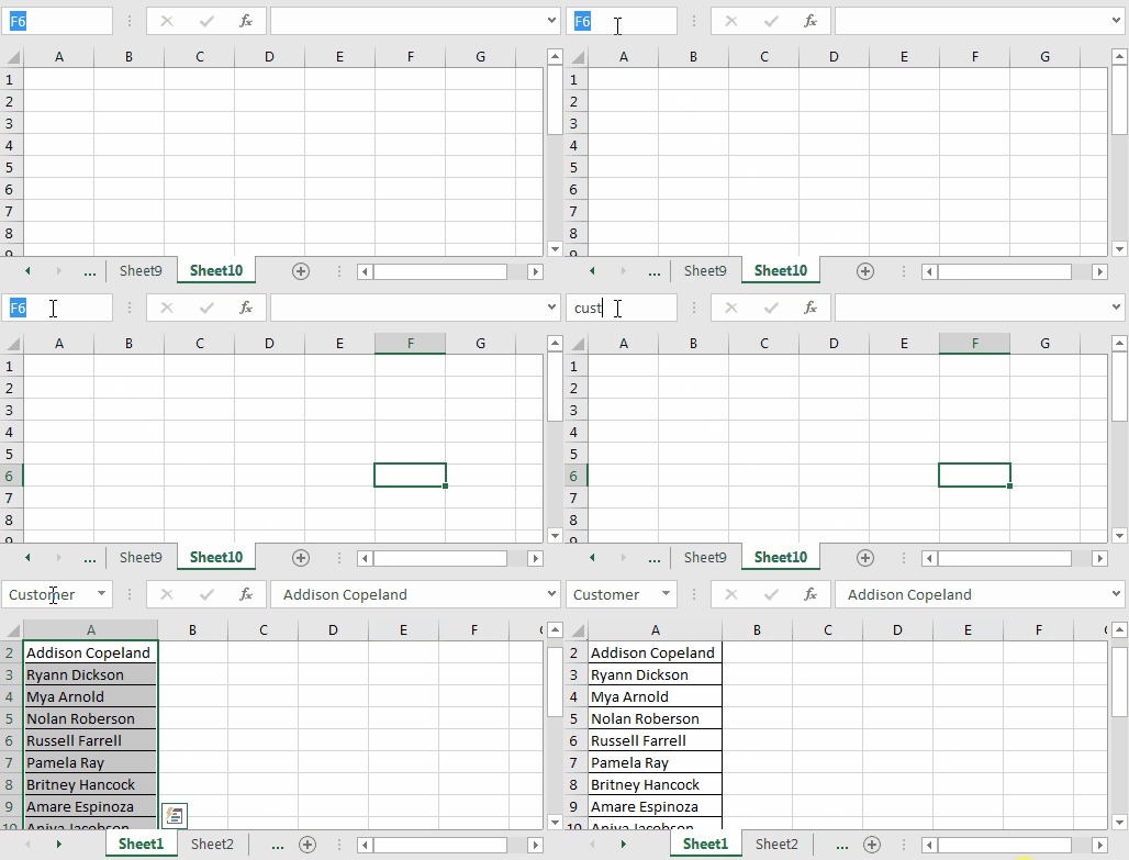
It will reduce the effort of remembering the ranges.
When your sheet is large and you often go from one point to another, you like to use hyperlinks in to navigate easily. Well Named Ranges can work perfectly with Hyperlinks. To add hyperlinks using named ranges follow these steps.


And its done. You have your hyperlink to your chosen named range. Using this you can create an index of named ranges that you can see and click to navigate to them directly. This will make your workbook really user friendly.
Named ranges and Data Validation is kind of made for each other. Named ranges make data validation highly customisable. It gets a lot easier to add a validation from a list using named range. Let us see how..

Now this cell will have names of customers who are part of Customer named range. Easy, isn’t it.
Now what if you want a cascading or dependent data validation. For example, if you you want a drop down list that has categories, Fruits and Vegetables. Now if you choose fruits than another drop down should show only fruits option and if you choose Vegetable then only vegetables.
This can be easily achieved by using Named ranges. Learn how.
Although Excel Tables provide structured names but they can not be used with data validation and Conditional Formatting. I don’t know why excel doesn’t allow it.
But it doesn’t mean that it can’t be done. You can name ranges within a table and then use them for validation. Excel does not have any problem with it.
So far we talked about named ranges that had Workbook scope. What? We we didn’t discussed it? Ok, so lets quickly understand what Scope of named ranges are.
Well scope defines where a name range can be recognised. Any name can not be recognised out its scope. For example a name in workbook1 can not be recognised in different workbook. Excel provides two options for scope of named ranges Worksheet and Workbook.
When you create a new name range, you can see a ‘Scope:’ section. Click on the drop down and choose the scope for your name range. You can’t change scope once you have created a named range. So better do it before. By default, it is workbook.
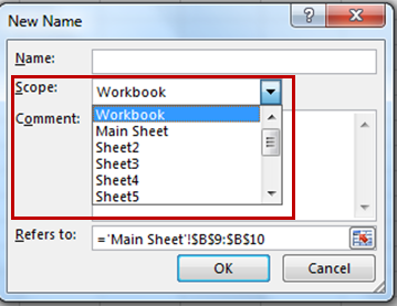
This is the default scope for a named range. A name defined with scope of workbook can be used in whole workbook in which it is defined (not other workbooks).
All above examples had workbook scope.
A name that is define with a worksheet scope can only be used on define worksheet. For example if I define ‘Total’ for a total cell with scope of sheet1. Then total will be recognised on sheet1 only. Other sheets will not recognise.
Excel does not have Global or say Excel Scope. Actually, I would like to define some names that can be recognised in all workbooks on my system. If anyone knows how can we do this, let me know.
You can’t. Excel does not allow you to edit scope of a named range once you have create. Since all named ranges on a sheet are by default Workbook Scoped, and you may want to change their scope to a sheet.
To do so, just make a copy of that sheet and excel will make each name on that sheet local to avoid ambiguity. You can now delete the original sheet if you like.
When you cut and paste a named range from one destination to another, the reference changes to new location. For example if you have a named range “Customer” in A2:A10 and cut and paste it to B2:B10, then customer name will refer to new location B2:B10.
Related Article:
17 Amazing Features of Excel Tables
Popular Articles:
50 Excel Shortcuts to Increase Your Productivity
How to use the VLOOKUP Function in Excel
The applications/code on this site are distributed as is and without warranties or liability. In no event shall the owner of the copyrights, or the authors of the applications/code be liable for any loss of profit, any problems or any damage resulting from the use or evaluation of the applications/code.