If Cell Contains Word then Assign Value in Microsoft Excel 2010

In this article we will learn if cell contains word then how to assign value in Microsoft Excel 2010.

Let's consider we have a situation where we need to review each cell and check if it contains any text.  If yes, we need to return a number in a separate cell, else ignore.  We can see how this is done using an example -

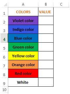
Column A has text containing the word “color”.  1 cell doesn’t.  (The colors are not of any significance here).  We need to check if each cell in this column contains the word “color”.  If it does, we need to return the value 1 in column B, else we need to return 0.

To understand better, see the below screenshot:

We will use 3 functions, namely, IF, SEARCH & IFERROR to calculate the value in column B.

The If function checks whether a condition is met, and returns one value if TRUE, and another if FALSE.

Syntax =IF(logical_test,value_if_true,value_if_false)

The SEARCH function returns the number of the character at which a specific character or text string is first found, reading left to right (not case-sensitive)

Syntax =SEARCH(find_text,within_text,start_num)

The IFERROR function returns value_if_error if expression is an error and the value of the expression itself otherwise

Syntax =IFERROR(value,value_if_error)

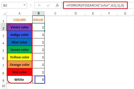
In cell B2, the formula is =IFERROR(IF(SEARCH("color",A2),1),0)

Refer below screenshot:

In cellsA2:A8 colors of the rainbow - VIBGYOR are used. To make things different in cell A9 White is entered since White is not part of VIBGYOR.

Hence, the result is 1 in cells A2:A8 since each of those cells contain the text “color” and 0 in cell A9 since it doesn’t contain the text “color” (see blue highlighted box above).

Let us understand how the formula works:

• Starting with cell A2, the Search function will look for the text “color” in this cell.  If found, it will return 8 which is the location at which the text was found in cell A2.  If the text is not found like in cell A9, then the function will return the #VALUE! Error.

• Then the IF function will check whether the search function returned any value.  If yes, it will return 1, else it will continue to return the #VALUE! error.

• Lastly, the IFERROR function will check if the search function has returned a #VALUE! Error and if yes, it will return a 0 instead of the error in that cell.