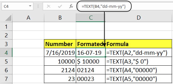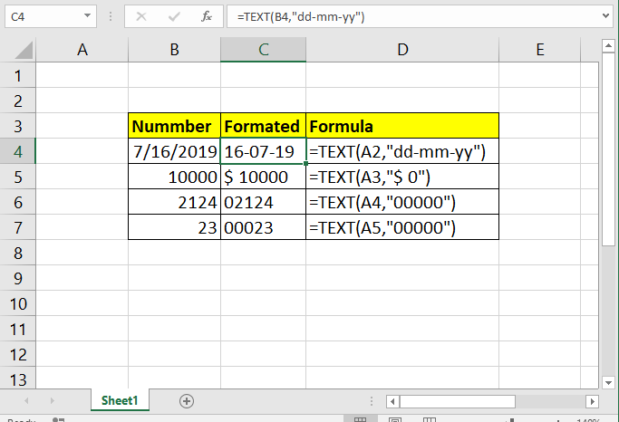
In this article, we will learn How to convert Numerically Calculated Results into One Output String and then combine them with different Text in Excel.
Scenario:
Excel treats values to many formats like number, date, time, text, percentage or currency. These can be changed into each other. Excel converts numbers to text to use numbers as text in formulas like vlookup with numbers and text. The Excel TEXT function lets you convert the number to text. The TEXT function in Excel is used to convert numbers into text. The fun part is you can format that number to show it in the desired format. For example format a yy-mm-dd date into dd-mm-yy format. Add currency signs before a number and many more.
TEXT formula in Excel
TEXT function is a string function which converts any value to a given format. The result may seem that it is a number but it's in text format.
| =TEXT(cell_ref, text_format) |
cell_ref : value to convert using cell reference
Text_format : Format to convert
| Format | Output_format |
| d | 7 |
| ddd | Thu |
| dddd | Thursday |
| m | 2 |
| mmm | Feb |
| mmmm | February |
| mmmmm | F |
| yy | 19 |
| yyyy | 2019 |
| m/d/y | 2/7/19 |
| mm/dd/yy | 02/07/19 |
| mm/dd/yyyy | 02/07/2019 |
| ddd, mmm d | Thu, Feb 7 |
| mm/dd/yyyy h:mm AM/PM | 02/07/2019 2:15 PM |
| mm/dd/yyyy hh:mm:ss | 07/02/2019 14:15:00 |
Example :
All of these might be confusing to understand. Let's understand how to use the function using an example. Here we have some examples to convert date values to text format or any other required format.

Convert the value in A2 cell.
Use the formula in C2 cell
| =TEXT (A2, “0”) |
“0”: returns the general text format.

Press Enter and copy the formula in remaining cells using Ctrl + D

As you can see we got numbers as text output because the significance number always varied.
Here we have some numbers to convert to text format or any other required format.
Use the formula:
| =TEXT(A2,"d") |

As you can see the value in the output cell is in Text format.

You can use any Format_text and do your work in excel without any interruption
Sometimes you are needed to add 0 before some fixed digit of numbers like phone number or pin number. Use this Text formula to do so…
| =TEXT( 1234, “00000”) |
If you have N digits of number then in text format argument write n+1 0s.
Write this text formula to add currency.
| =TEXT( 1234, “$0”) |

As you can see we got numbers as text output because the significance number always varied.
VBA Code to convert currency in TEXT format
This code is divided into four individual functions. The main function is NUM_TO_IND_RUPEE_WORD. And other three functions GetHunderds(), GetTens() and GetDigits are helping function that help the main function to form the string.
Code
| Function NUM_TO_IND_RUPEE_WORD(ByVal MyNumber, Optional incRupees As Boolean = True)
Dim Crores, Lakhs, Rupees, Paise, Temp Dim DecimalPlace As Long, Count As Long Dim myLakhs, myCrores ReDim Place(9) As String Place(2) = " Thousand ": Place(3) = " Million " Place(4) = " Billion ": Place(5) = " Trillion "
' String representation of amount. MyNumber = Trim(Str(MyNumber))
' Position of decimal place 0 if none. DecimalPlace = InStr(MyNumber, ".")
' Convert Paise and set MyNumber to Rupees amount. If DecimalPlace > 0 Then Paise = GetTens(Left(Mid(MyNumber, DecimalPlace + 1) & "00", 2)) MyNumber = Trim(Left(MyNumber, DecimalPlace - 1)) End If
myCrores = MyNumber \ 10000000 myLakhs = (MyNumber - myCrores * 10000000) \ 100000 MyNumber = MyNumber - myCrores * 10000000 - myLakhs * 100000 Count = 1
Do While myCrores <> "" Temp = GetHundreds(Right(myCrores, 3)) If Temp <> "" Then Crores = Temp & Place(Count) & Crores If Len(myCrores) > 3 Then myCrores = Left(myCrores, Len(myCrores) - 3) Else myCrores = "" End If Count = Count + 1 Loop Count = 1
Do While myLakhs <> "" Temp = GetHundreds(Right(myLakhs, 3)) If Temp <> "" Then Lakhs = Temp & Place(Count) & Lakhs If Len(myLakhs) > 3 Then myLakhs = Left(myLakhs, Len(myLakhs) - 3) Else myLakhs = "" End If Count = Count + 1 Loop Count = 1
Do While MyNumber <> "" Temp = GetHundreds(Right(MyNumber, 3)) If Temp <> "" Then Rupees = Temp & Place(Count) & Rupees If Len(MyNumber) > 3 Then MyNumber = Left(MyNumber, Len(MyNumber) - 3) Else MyNumber = "" End If Count = Count + 1 Loop
Select Case Crores Case "": Crores = "" Case "One": Crores = " One Crore " Case Else: Crores = Crores & " Crores " End Select Select Case Lakhs Case "": Lakhs = "" Case "One": Lakhs = " One Lakh " Case Else: Lakhs = Lakhs & " Lakhs " End Select Select Case Rupees Case "": Rupees = "Zero " Case "One": Rupees = "One " Case Else: Rupees = Rupees End Select Select Case Paise Case "": Paise = " and Paise Zero Only " Case "One": Paise = " and Paise One Only " Case Else: Paise = " and Paise " & Paise & " Only " End Select 'creating the string of words to translate number into words NUM_TO_IND_RUPEE_WORD = IIf(incRupees, "Rupees ", "") & Crores & _ Lakhs & Rupees & Paise End Function ' Converts a number from 100-999 into text Function GetHundreds(ByVal MyNumber) Dim Result As String If Val(MyNumber) = 0 Then Exit Function MyNumber = Right("000" & MyNumber, 3) ' Convert the hundreds place. If Mid(MyNumber, 1, 1) <> "0" Then Result = GetDigit(Mid(MyNumber, 1, 1)) & " Hundred " End If ' Convert the tens and ones place. If Mid(MyNumber, 2, 1) <> "0" Then Result = Result & GetTens(Mid(MyNumber, 2)) Else Result = Result & GetDigit(Mid(MyNumber, 3)) End If GetHundreds = Result End Function ' Converts a number from 10 to 99 into text. Function GetTens(TensText) Dim Result As String Result = "" ' Null out the temporary function value. If Val(Left(TensText, 1)) = 1 Then ' If value between 10-19... Select Case Val(TensText) Case 10: Result = "Ten" Case 11: Result = "Eleven" Case 12: Result = "Twelve" Case 13: Result = "Thirteen" Case 14: Result = "Fourteen" Case 15: Result = "Fifteen" Case 16: Result = "Sixteen" Case 17: Result = "Seventeen" Case 18: Result = "Eighteen" Case 19: Result = "Nineteen" Case Else End Select Else ' If value between 20-99... Select Case Val(Left(TensText, 1)) Case 2: Result = "Twenty " Case 3: Result = "Thirty " Case 4: Result = "Forty " Case 5: Result = "Fifty " Case 6: Result = "Sixty " Case 7: Result = "Seventy " Case 8: Result = "Eighty " Case 9: Result = "Ninety " Case Else End Select Result = Result & GetDigit _ (Right(TensText, 1)) ' Retrieve ones place. End If GetTens = Result End Function ' Converts a number from 1 to 9 into text. Function GetDigit(Digit) Select Case Val(Digit) Case 1: GetDigit = "One" Case 2: GetDigit = "Two" Case 3: GetDigit = "Three" Case 4: GetDigit = "Four" Case 5: GetDigit = "Five" Case 6: GetDigit = "Six" Case 7: GetDigit = "Seven" Case 8: GetDigit = "Eight" Case 9: GetDigit = "Nine" Case Else: GetDigit = "" End Select End Function |
The above code will get the result in correct format. Now make your own customized function.
For example, you can use the following formula to return the current date:
| =CONCATENATE("Today is ",TEXT(TODAY(), "dd-mmm-yy")) |

Using CONCATENATE in Excel - things to remember
To ensure that your CONCATENATE formulas always deliver the correct results, remember the following simple rules:
Excel CONCATENATE function requires at least one "text" argument to work.
Here are all the observational notes using the formula in Excel
Notes :
Hope this article about How to Combine Text and Numerically Calculated Results into One Output String in Microsoft Excel is explanatory. Find more articles on calculating values and related Excel formulas here. If you liked our blogs, share them with your friends on Facebook. And also you can follow us on Twitter and Facebook. We would love to hear from you, do let us know how we can improve, complement or innovate our work and make it better for you. Write to us at info@exceltip.com.
Related Articles :
Excel REPLACE vs SUBSTITUTE function: The REPLACE and SUBSTITUTE functions are the most misunderstood functions. To find and replace a given text we use the SUBSTITUTE function. Where REPLACE is used to replace a number of characters in a string.
How to use the ISTEXT function in Excel : returns the TRUE logic value if the cell value is text using the ISTEXT function in Excel.
How to Highlight cells that contain specific text in Excel : Highlight cells based on the formula to find the specific text value within the cell in Excel.
Converts decimal Seconds into time format : As we know that time in excel is treated as numbers. Hours, Minutes, and Seconds are treated as decimal numbers. So when we have seconds as numbers, how do we convert into time format? This article got it covered.
Calculate Minutes Between Dates & Time in Excel : calculating the time difference is quite easy. Just need to subtract the start time from the end time. Learn more about this formula clicking the link
Replace text from end of a string starting from variable position : To replace text from the end of the string, we use the REPLACE function. The REPLACE function use the position of text in the string to replace.
Popular Articles :
50 Excel Shortcuts to Increase Your Productivity : Get faster at your tasks in Excel. These shortcuts will help you increase your work efficiency in Excel.
How to use the VLOOKUP Function in Excel : This is one of the most used and popular functions of excel that is used to lookup value from different ranges and sheets.
How to use the IF Function in Excel : The IF statement in Excel checks the condition and returns a specific value if the condition is TRUE or returns another specific value if FALSE.
How to use the SUMIF Function in Excel : This is another dashboard essential function. This helps you sum up values on specific conditions.
How to use the COUNTIF Function in Excel : Count values with conditions using this amazing function. You don't need to filter your data to count specific values. Countif function is essential to prepare your dashboard.
The applications/code on this site are distributed as is and without warranties or liability. In no event shall the owner of the copyrights, or the authors of the applications/code be liable for any loss of profit, any problems or any damage resulting from the use or evaluation of the applications/code.
If you're having trouble with the formula, make sure to use straight quotes unlike the article which uses left/right double quotes.
C2 =TEXT(A2,”MMMM”)
?
C2 =TEXT(A2,"MMMM")
That's right.
thanks