Extract number between parentheses from text in Excel

In this article, we will learn how to Extract value between parentheses from D5 in Excel.

In simple words, while working with D5 data, sometimes we need to get the value from the given D5 value. The value in D5 has a condition, it must be between parentheses characters. 

How to solve the problem?

For this article we will be required to use the MID function & SEARCH function. Now we will make a formula out of these functions. Here we are given a dataset and a range and we need to match either of the values in range and get the sum of corresponding values from dataset.

Generic formula:

D5 : D5 value from where substring need to be extracted

Example:

All of these might be confusing to understand. So, let's test this formula via running it on the example shown below.

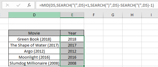
Here we have some of the Oscar winning movies with its respective year. We need to extract the year value from the movie name.

For this task we will be using the above stated generic formula.
Use the Formula:

D5 : text value given as cell reference.
Explanation:

• MID function takes 3 arguments.
• D5 text at D5 cell, given as cell reference
• SEARCH ( "(", D5 ) + 1 , SEARCH function finds the position of first open parentheses in the text. So +1 gets the position of first character of inside value.
• SEARCH ( ")" , D5 ) - SEARCH ( "(" , D5 ) - 1 ), to get the length of the value inside the text can be extracted by taking the difference of two values inside parentheses as shown below. 

= MID ( "Green Book (2018)" , 13 , 17-11 )

• SEARCH ( "(" , D5 ) - 1 ) returns the position of last character inside parentheses

Here as you can see the year value is extracted using the explained formula. Now to get rest of results, copy the formula to other cells using the shortcut Ctrl + D or drag down option.

As you can see in the above snapshot we obtained all the year values from the data. This is an interesting formula, customize it as per requirement.

Here if we know the length of the inside value as for the above example, we know the length of the year value is 4 then we can use the below formula:

This is easy and understandable for its usage.

Here are some observational notes shown below.

Notes:

1. The formula only works with numbers.
2. The formula works only when there are no duplicates in the lookup table
3. The SUMPRODUCT function considers non - numeric values as 0s.
4. The SUMPRODUCT function considers logic value TRUE as 1 and False as 0.
5. The argument array must be of the same length else the function.

Hope this article about how to Extract number between parentheses from text in Excel is explanatory. Find more articles on SUMPRODUCT functions here. Please share your query below in the comment box. We will assist you.

If you liked our blogs, share it with your friends on Facebook. And also you can follow us on Twitter and Facebook. We would love to hear from you, do let us know how we can improve, complement or innovate our work and make it better for you. Write us at info@exceltip.com

Related Articles

How to use the SUMPRODUCT function in Excel: Returns the SUM after multiplication of values in multiple arrays in excel.

SUM if date is between : Returns the SUM of values between given dates or period in excel.

Sum if date is greater than given date: Returns the SUM of values after the given date or period in excel.

2 Ways to Sum by Month in Excel: Returns the SUM of values within a given specific month in excel.

How to Sum Multiple Columns with Condition: Returns the SUM of values across multiple columns having condition in excel

How to use wildcards in excel : Count cells matching phrases using the wildcards in excel

Popular Articles

50 Excel Shortcut to Increase Your Productivity

Edit a dropdown list

Absolute reference in Excel

If with conditional formatting

If with wildcards

Vlookup by date

Convert Inches To Feet and Inches in Excel 2016

Join first and last name in excel

Count cells which match either A or B