Retrieve Value Using Case-Sensitive "Lookup" in Microsoft Excel 2010

If you want a formula that will return the value using case sensitive lookup,you can use a combination of "INDEX"," MATCH" & "EXACT" functions to derive the output.
INDEX: Returns a value or reference of the cell at the intersection of a particular row and column, in a given range.

Syntax: =INDEX(array,row_num,column_num)

array:Array is a range of cells or table.

row_num:The row number in the array from which the value is returned.

column_num:It is optional. It is the column number in the array that is used to return the value.
MATCH function searches for a specified item in a selected range of cells, and then returns the relative position of that item in the range.

Syntax =MATCH(lookup_value,lookup_array,match_type)

lookup_value: The value you want to look for

lookup_array: The table of data contains information from which you want to return the output.

match_type: 1,0 and -1 are three options.

1(Default): It will find the largest value in the range. List must be sorted in ascending order.

0: It will find an exact match

-1: It will find the smallest value in the range. List must be sorted in descending order.
EXACT: Checks whether two text strings are exactly the same, and returns TRUE or FALSE. EXACT is case-sensitive.

Syntax =EXACT(text1,text2)

text1: Itis the first text string

text2: It is the second text string
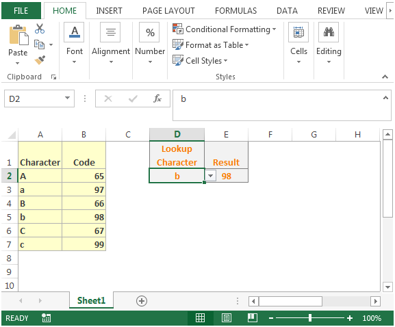
Let us take an example:

We have some characters in column A & their codes in column B using Code function.

In cell E2, we want a formula based on the lookup value in cell D2
The formula in cell E2 would be {=INDEX($B$2:$B$7,MATCH(TRUE,EXACT(D2,$A$2:$A$7),0))}
This is an array formula that has to be entered with CTRL + SHIFT + ENTER otherwise it will give false results

In cell D2, we have to apply drop down using Data Validation feature.
If we change the value in cell D2 to say b, the formula will return the value accordingly.