Retrieving the Row Number that Corresponds with a Matched Value in a Look Up in Excel 2010

To retrieve the row number which corresponds with a matched value in a lookup, we use the MAX function, along with the IF and ROW functions in Microsoft Excel 2010.

MAX: This function is used to return the largest number in a set of values. It ignores logical values and text.

Syntax of “MAX” function:            =MAX(number1, [number2],….)

Example: Range A1:A4contains a list of numbers and we need to return the maximum number.

Follow the below given steps:-

• Select the cell B1 and write the formula.
• =MAX(A1:A4), press Enter on your keyboard.
• The function will return 9.
• Hence 9 is the maximum value in the range A1:A4.

SMALL: - This function is used to return the k-th smallest value in a data set.

Syntax of “SMALL” function:         =SMALL (array,k)

Example:Column A contains few numbers, we want to find out the smallest number form the list.

• Select the cell B1.
• Write the formula =SMALL(A1:A4,1)
• Press Enter on your keyboard.
• The function will return smallest number in the row.

IF: - Checks whether a condition is met and returns one value if True and another value if False.

Syntax of “IF” function =if(logical test,[value_if_true],[value_if_false])

The function will perform a logical test and give the result based on whether its true or false.

For example: Cells A2 and A3 contain the numbers 3 and 5. If the cell contains 3, then the formula should display “Yes” otherwise “No”.

=IF (A1=3,"Yes","No")

ROW: - This function is used to return the row number of a cell reference.

Syntax of “ROW” function:           =ROW (reference)

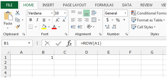
Example: =ROW (A1) would return 1

               =ROW (A1:A10) would return 1

              =ROW (A1:C10) would return 1  

Lets see how we can use the MAX function to pick the number, the IF function will check the logical test and the ROW function will identify the row number that corresponds with a matched value in a lookup.

Let’s take an example to understand how we can retrieve the row number that corresponds with a matched value in a lookup.

To retrieve the row number, we will use the MAX function, along with the IF and ROW functions in Microsoft Excel 2010 and 2013.

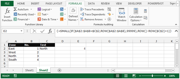
We need to search List 1 (column A) for each of the text in column C and retrieve the corresponding row number.  In this case, we need to compare the lookup value given in C2 with each entry in column A and find its corresponding row number. This row number has to be returned in E2.

Follow the below given steps:-

• Select the cell E2.
• Write the formula to retrieve the corresponding row number.
• =MAX(IF($A$2:$A$5=C2,ROW($A$2:$A$5)))
• Press Ctrl+Shift+Enteron the keyboard

• The function will retrieve the row number that corresponds with a matched value in lookup.

Note:- If we change the lookup value, the result will be changed automatically.  See the below screenshot – The lookup value has been changed to West, and its corresponding result which is 3 is showing in cell E2.

We can use another formula, to get the same result, follow the below given steps

• Select the cell E2.
• Write the formula to retrieve the corresponding row number.
• =SMALL(IF($A$2:$A$8=$C$2,ROW($A$2:$A$8),99999),ROW()-ROW($C$2)+1)
• Press Ctrl+Shift+Enter on the keyboard
• The formula will look like this - {=SMALL(IF($A$2:$A$8=$C$2,ROW($A$2:$A$8),99999),ROW()-ROW($C$2)+1)}

• The function will retrieve each row number which corresponds with a successful matchto the lookup value.