Set up conditional formatting for an area using VBA in Microsoft Excel

In this article, we will create a macro to apply conditional formatting in the selected area.

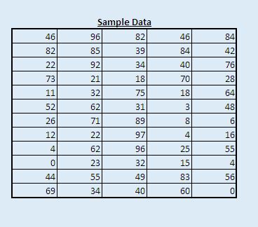
We have used random numbers as sample data to demonstrate working of the macro.

RawData

Macro can be executed by clicking “Find Max” button on “Main” sheet.

ArrowMainSheet

Logic explanation

We have created “ConditionalFormat” macro to apply conditional formatting to the selected area. This macro highlights the cell in violet color, which contains the maximum value in the selected area.

Before executing this macro, one has to select an area on which he wants to apply the conditional formatting.

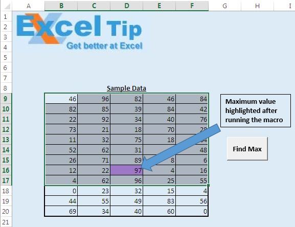
For example, we have selected a range of cells from B9 to F17 as the sample of selected data.

ArrowSelectedSample

On executing the macro after selecting sample area, conditional formatting is applied on the selected area and cell D16, which contains the highest value (97), will be highlighted in violet color.

ArrowFirstSampleOutput

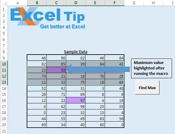
Now, take another sample. We have selected the range from cell B10 to F13 as second sample area.

ArrowSecondSample

After selecting the second sample area, click on “Find Max” button to run the macro. Conditional formatting will be applied on the selected area and cell C11 will be highlighted in violet color, as it contains the maximum value (92) in the selected area.

ArrowSecondSampleOutput

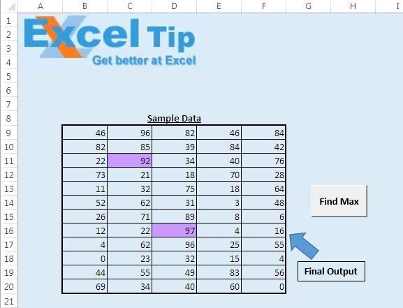
After executing the macro for two different samples, conditional formatting is applied to both of them. In the sample data, both the cells C11 and D16 will be highlighted in violet color, as they represent maximum values in their respective samples.

ArrowFinalOutput

If values in any of the samples are changed and one of the newly inserted values is the highest value, then the cell with that particular value will be highlighted.

Code explanation

Selection.FormatConditions.Delete

Above code is used to delete any conditional formatting applied on the selected data.

Selection.FormatConditions.Add Type:=xlExpression, Formula1:= _

"=" & Selection.Cells(1).Address(False, False) & "=MAX(" & Selection.Address & ")"

Above code is used to add a new conditional formatting. Type specifies that expression is used to apply the condition formatting. Formula of the expression is defined in Formula1.

Selection.Cells(1).Address(False, False)

Above code is used to reference address of the first cell in the selection.

"=" & Selection.Cells(1).Address(False, False) & "=MAX(" & Selection.Address & ")"

Above code is used to compare the value of the first selected cell with the maximum value of the selection.

Selection.FormatConditions(1).Interior.ColorIndex = 39

Above code is used to assign violet color to the cell that satisfies the condition of the formatting.

Please follow below for the code


Sub ConditionalFormat()

With Selection
    'Delete any previous conditional formatting
    .FormatConditions.Delete
    
    'add conditional formatting to selected cell
    .FormatConditions.Add Type:=xlExpression, Formula1:= _
    "=" & Selection.Cells(1).Address(False, False) & "=MAX(" & Selection.Address & ")"
    
    'Assigning Violet color for the conditional formatting
    .FormatConditions(1).Interior.ColorIndex = 39
    
End With
   
   
End Sub

If you liked this blog, share it with your friends on Facebook. Also, you can follow us on Twitter and Facebook.

We would love to hear from you, do let us know how we can improve our work and make it better for you. Write to us at info@exceltip.com