In this article, we are going to learn how to ignore the N/A error in result while using Vlookup function in Microsoft Excel.
As we all know that IFERROR function is used for providing the output as result when any error occurs while calculation.
And, VLOOKUP function is used for retrieving the data information in first data to another data on the basis of common value. So when the common value not matched with the second data then formula give us #N/A error as output.
Let’s take an example to understand how we can ignore VLOOKUP #N/A Error in Excel.
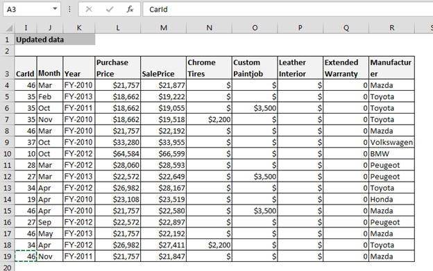
We have 2 data sets. 1st is main data and 2nd is updated data. Now, we want to update the main data from the updated data.
Main Data:-
Updated Data:-

In the main data, we want to update the manufacturer details from the updated sheet.
Follow below given steps:-
This is the way we can eliminate NA error as result when using VLOOKUP formula in Microsoft Excel.
If you liked our blogs, share it with your friends on Facebook. And also you can follow us on Twitter and Facebook.
We would love to hear from you, do let us know how we can improve, complement or innovate our work and make it better for you. Write us at info@exceltip.com
The applications/code on this site are distributed as is and without warranties or liability. In no event shall the owner of the copyrights, or the authors of the applications/code be liable for any loss of profit, any problems or any damage resulting from the use or evaluation of the applications/code.
This tip worked just as written - thanks for saving me hours of time trying to fiture this out by myself!!!