Calculate marks with criteria in Excel

In this article, we will learn how to calculate total marks with criteria in Excel.

Scenario:

For instance, while working with the correct and response key in dataset. Sometimes given a condition i.e. when we need to get the marks for the correct answer and wrong answers and no response. You can perform the solution to this problem easily using the excel functions as explained below.

How to solve the problem?

For this article we will be required to use the SUM function or SUMPRODUCT function. Now we will make a formula out of the mentioned functions. Here we are given a list of correct answers and a list of the student responses. We need to find the SUM of the correct marks and wrong marks. 

Generic formula for correct responses:

Note : DO NOT use curly braces manually. Curly braces are applied using the Ctrl + Shift + Enter in place of just Enter as it is an array formula.

OR

response : range of answers as response

correct_list : the correct response for the questions.

Example:

All of these might be confusing to understand. So, let's test this formula via running it on the example shown below.

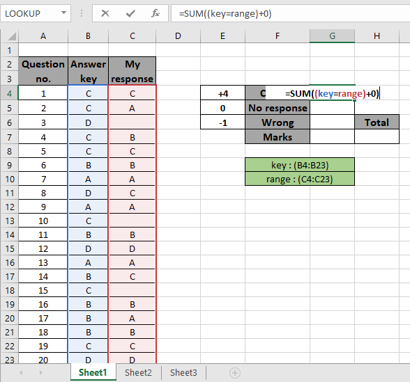
Here we have a list of question numbers and answer key corresponding to it. Then along with that we have a list of student responses as my response. The marks criteria is based on the given values as +4 for correct answer and -1 for wrong answer and 0 for no response.

Here are the named ranges used to provide a fixed array to the formula. Named ranges are mentioned in green boxes.

Firstly,  we need to find the marks for the correct responses.

Use the Formula:

DO NOT use curly braces manually. Curly braces applied using the Ctrl + Shift + Enter in place of just Enter.

Explanation:

• Key = range matches all the correct responses and returns the array of TRUEs and FALSEs to the SUM function.
• +0 will return the resulting count in numbers format.
• SUM function finds the sum for the TRUE values and TRUE as 1 and FALSE as 0.

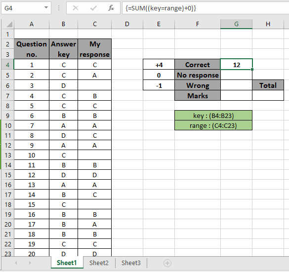
Press Ctrl + Shift + Enter to get the SUM of the required values as this is an array formula.

As you can see in the above snapshot that sum of correct answers which comes out to be 12. Now get how many were the answers were left as no response. For this we use COUNTBLANK function as no response gets blank cells.

Use the Formula:

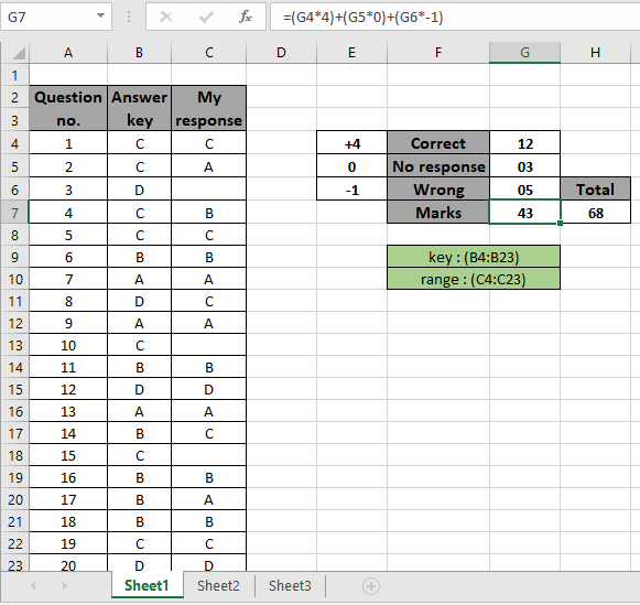
There are 3 blanks in the range which gives us no response count. Now to get the number of wrong answers count we will find the answers which don't match the given response to the question.

Use the Formula:

Explanation:

• Key <> range matches all the unmatched responses and returns the array of TRUEs and FALSEs to the SUMPRODUCT function.
• SUMPRODUCT ( ( key <> range ) + 0 ) will returns all the unmatched responses including blank ones.
• Subtract the blank responses as we considered it already.

Press Enter to get the result.

Here the wrong response count. Now to calculate the marks we will use the below mathematical formulation.

Use the Formula:

As we know the correct response gets 4 marks , 0 for no response and -1 for wrong response.

We got the marks obtained as 43 out of total marks which are 68.  

Here are some observational notes shown below.

Notes:

1. The formula only works with numbers.
2. The formula works only when there are no duplicates in the list & code table.
3. The MATCH function takes 0 as an argument to get the exact match from the list.
4. DONOT use curly braces manually. Curly braces applied using the Ctrl + Shift + Enter in place of just Enter as it is an array formula.
5. The list array length must be of the same as the code length else the function.

Hope this article about how to Calculate total marks with criteria in Excel is explanatory. Find more articles on SUMPRODUCT functions here. Please share your query below in the comment box. We will assist you. If you liked our blogs, share it with your friends on Facebook. And also you can follow us on Twitter and Facebook. We would love to hear from you, do let us know how we can improve, complement or innovate our work and make it better for you. Write us at info@exceltip.com

Related Articles

How to use the SUMPRODUCT function in Excel: Returns the SUM after multiplication of values in multiple arrays in excel.

SUM if date is between : Returns the SUM of values between given dates or period in excel.

Sum if date is greater than given date: Returns the SUM of values after the given date or period in excel.

2 Ways to Sum by Month in Excel: Returns the SUM of values within a given specific month in excel.

How to Sum Multiple Columns with Condition: Returns the SUM of values across multiple columns having condition in excel

How to use wildcards in excel : Count cells matching phrases using the wildcards in excel

Popular Articles

50 Excel Shortcut to Increase Your Productivity

Edit a dropdown list

Absolute reference in Excel

If with conditional formatting

If with wildcards

Vlookup by date

Convert Inches To Feet and Inches in Excel 2016

Join first and last name in excel

Count cells which match either A or B