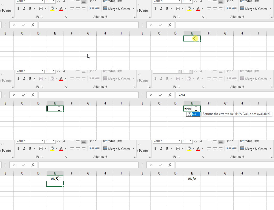
In this article, we will learn about how to use the NA function in Excel.
In simple words, this function is used with other functions to accept the condition and give response to the user as desired
The NA function returns a not applicable error when used with other functions.
Syntax:
Returns the error

Let’s understand this function using it in an example.

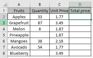
We need to find out the Total price for all the fruits and do not want 0 in return.
We will use the formula:
B2 = “” : condition to check for empty cells that we will return 0
NA() : value if condition is True.
B2*C2 : value if condition is False

As you can see the value if condition is False.
Now copy the formula in other cells using shortcut key Ctrl + D.

As you can see the formula returns value error where condition stands True
Hope you understood how to use the NA function in Excel. Explore more articles on Excel logic_test functions here. Please feel free to state your query or feedback for the above article.
Related Articles:
How to Use IFERROR function in Excel
How to Use ISERROR Function in Excel
Popular Articles:
How to use the VLOOKUP Function in Excel
The applications/code on this site are distributed as is and without warranties or liability. In no event shall the owner of the copyrights, or the authors of the applications/code be liable for any loss of profit, any problems or any damage resulting from the use or evaluation of the applications/code.