How to use the N Function in Excel

In this article, we will learn the function N in Excel.

N function returns number as per the input value. The conversion is usually to use the values for further formulation. See below table for more understanding of the function.

Input	Return
Number	Same number
Date or Time	Serial number format
TRUE	1
FALSE	0
Error code	Same error code
Text or other values	0

N function returns 1 for TRUE logic value and 0 for FALSE logic value.

N function converts the value to a number.
Syntax:

=N ( value )

value : value to the function can be given as directly or using cell reference

Now let’s understand the function more via using it in an example

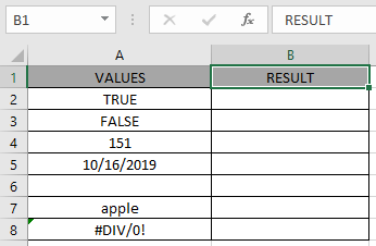
Here we have a list of value in Column A & we need to check the cells for the TEXT values.

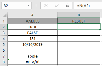
Use the formula:

= N ( A2 )

A2 : reference cell is provided to the function to check its value.

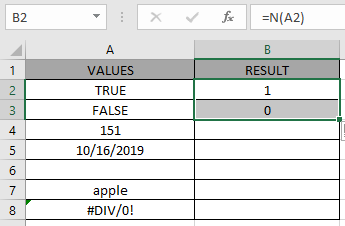
And now the result of A3 cell.

You can observe the difference in output from the above snapshots between the LOGIC values.

Copy the formula to other cells using the Ctrl + D shortcut key.

As you can see, the function returns a number
Note:

When range of cells given as argument, the function only checks the first cell of the array as returns TRUE or FALSE based only on the first cell.
The function returns 1 for TRUE logical value but returns 0 for FALSE.

Hope you understood how to use N function in Excel 2016. Find more articles on Excel N function here. Please share your query below in the comment box. We will assist you.