As I have mentioned in many of my blogs that a SUMPRODUCT is a very versatile function and can be used for multiple purposes. In this article, we will see how we can use this function to count values with multiple OR criteria.
Generic SUMPRODUCT Formula to Count With Multiple Or Criteria
| =SUMPRODUCT(--(((criteria1)+(criteria2)+...)>0) |
Criteria1: This is any criteria that returns an array of TRUE and FALSE.
Criteria2: This is the next criteria that you want to check. Similarly, you can have as many criteria as you want.
The above generic formula is modified often to suit the requirements to count with multiple OR criteria. But the base formula is this. First we will see how this works through an example and after that we will discuss other scenarios where you will need to modify this formula a little.
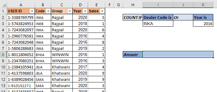
So here we have a data set of salespeople. The data contains many columns. What we need to do is to count the number of users who have code "INKA" or year is "2016". Make sure that if someone has both (code as "inka" and year 2016) it should be counted as 1.
So, here we have two criteria. We use the above mentioned SUMPRODUCT formula:
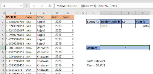
| =SUMPRODUCT(--(((Code=I3)+(Year=K3))>0)) |
Here, code and year are named ranges.
This returns 7.
In the data we have 5 records of INKA code and 4 records of year 2016. But 2 records have both "INKA" and 2016 as code and year respectively. These records are counted as 1. And this is how we get 7.
How does it work?
So let's have a look at how the formula is solved step by step, then I will discuss how it works.
| =SUMPRODUCT(--(((Code=I3)+(Year=K3))>0)) |
| 1=>SUMPRODUCT(--(({TRUE;FALSE;TRUE;TRUE;TRUE;TRUE;...}+{FALSE;FALSE;FALSE;TRUE;TRUE;...})>0)) |
| 2=>SUMPRODUCT(--(({1;0;1;2;2;1;1;1;0;0;0;0;0;0;0;0;0;0;0;0})>0)) |
| 3=>SUMPRODUCT(--({TRUE;FALSE;TRUE;TRUE;TRUE;TRUE;TRUE;...}) |
| 4=>SUMPRODUCT({1;0;1;1;1;1;1;1;0;0;0;0;0;0;0;0;0;0;0;0}) |
| 5=>7 |
In the first step, the value of I3 ("INKA") is compared with each cell in the code range. This returns an array of TRUE and FALSE. TRUE for each match. To save space I have not shown all TRUE-FALSE. Similarly, the value of K3 (2016) is matched with each cell in the year range.
In the next step, we add these two arrays that result in a new array of numeric values. As you may know, TRUE is treated as 1 and FALSE as 0 in Excel. So when TRUE and TRUE are added we get 2 and the rest you can understand.
In the next step, we check which value is greater than 0 in the array. This again converts the array into a true false array. For each 0 value we get, False and rest are converted as true. Now the number of TRUE values in the array is our answer. But how do we count them? Here's how.
Double negative (--) signs are used to convert boolean values into 1s and 0s. So each TRUE value in the array is converted into 1 and FALSE into 0.
In the final step the SUMPRODUCT sums up this array and we get our answer as 7.
So if you need to add more or criteria to count, you can just add criteria using + sign to the function.
For example, if you want to add another criteria to the above formula so that it adds the number of employees who have sold more than 5 products. The SUMPRODUCT formula will simply look like this:
| =SUMPRODUCT(--(((Code=I3)+(Year=K3)+(Sales>5))>0)) |
Simple! isn't it?
But let's say you want to have two criteria from Code range. Let's say you want to count "INKB". So how do you do this? One method is using the above technique but that would be repetitive. Let's say I want to add 10 more criteria from the same range. In such cases this technique is not that smart for counting with SUMPRODUCT.
Let's say we have data arranged like this.
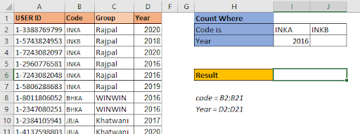
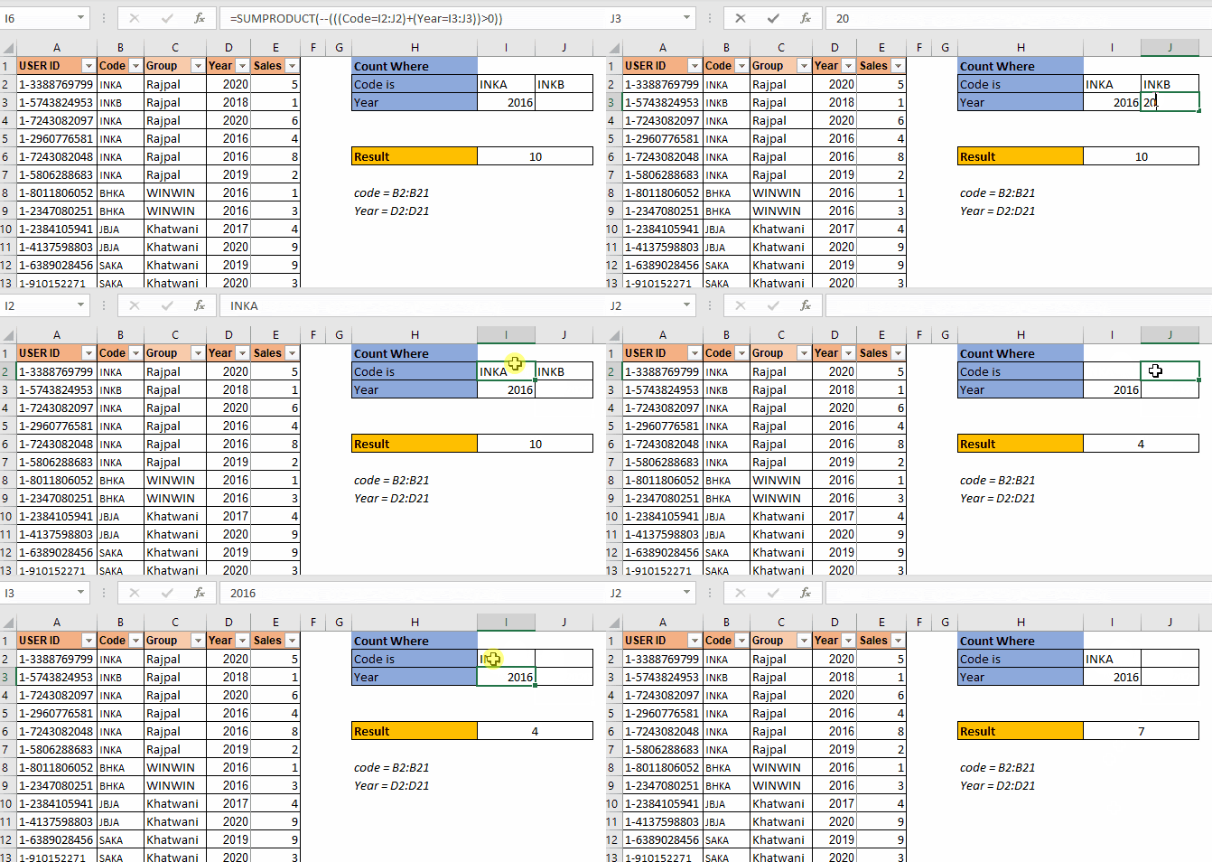
The criteria codes are in one row I2:J2. The arrangement of data is important here. The SUMPRODUCT formula for 3 OR criteria count settings will be:
| =SUMPRODUCT(--(((Code=I2:J2)+(Year=I3:J3))>0)) |
This is the SUMPRODUCT formula to count with multiple criteria when multiple criteria from one range are written in a row.
This returns the correct answer which is 10.
If you type any year in J3, the formula will add that count too.

This is used when the criteria are in one row. Will it work when the criteria are in one column for the same range? No. It won't.
In this example we have multiple codes to count but these type codes are written in one column. When we use the above SUMPRODUCT formula, we get ans #N/A error. We will not get into how this error came about as this will make this article too long. Let's see how we can make this work.

To make this formula work, you need to wrap the code criteria in TRANSPOSE function. This will get the formula working.
| =SUMPRODUCT(--(((Code=TRANSPOSE(H3:H4))+(Year=TRANSPOSE(I3:I4)))>0)) |
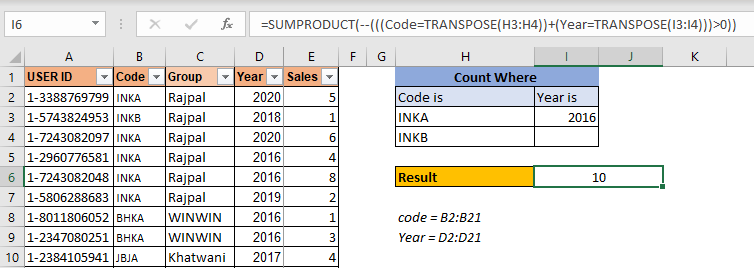
This is the formula for counting with multiple or conditions in the same range when criteria is listed in a column.
So yeah mate, I hope I was clear enough and it made sense. I hope it serves your purpose of being here. If this formula didn't solve your problem, let me know your requirements in the comments section below. I will be more than happy to help you in any way. You can mention any doubt related Excel/VBA. Till then keep learning, keep excelling.
Related Articles
How to use the SUMPRODUCT function in Excel: Returns the SUM after multiplication of values in multiple arrays in excel. This function can be used to do multiple tasks. This is one of the most versatile functions.
COUNTIFS with Dynamic Criteria Range : To count with dynamic criteria range we simply use the INDIRECT function. This function can
COUNTIFS With OR For Multiple Criteria : Count cells that have multiple criteria that match using the OR function. To put an OR logic in COUNTIFS function you will not need to use the OR function.
Using the IF with AND / OR Functions in Microsoft Excel : These logical functions are used to carry out multiple criteria calculations. With IF the OR and AND functions are used to include or exclude matches.
How to use OR function in Microsoft Excel : The function is used to include all the TRUE values in multiple criterias.
How to Count Cells That Contain This Or That in Excel in Excel :To cells that contain this or that, we can use the SUMPRODUCT function. Here's how you do those calculations.
Popular Articles:
50 Excel Shortcuts to Increase Your Productivity | Get faster at your task. These 50 shortcuts will make you work even faster on Excel.
How to use Excel VLOOKUP Function| This is one of the most used and popular functions of excel that is used to lookup value from different ranges and sheets.
How to use the Excel COUNTIF Function| Count values with conditions using this amazing function. You don't need to filter your data to count specific values. Countif function is essential to prepare your dashboard.
How to Use SUMIF Function in Excel | This is another dashboard essential function. This helps you sum up values on specific conditions.
The applications/code on this site are distributed as is and without warranties or liability. In no event shall the owner of the copyrights, or the authors of the applications/code be liable for any loss of profit, any problems or any damage resulting from the use or evaluation of the applications/code.