Ok, so in my early days of data analysis, I got a need to automatically get the unique items in excel from a list, rather than removing duplicated each time. And I figured out a way to do it. After that my excel dashboard was even more dynamic than before. So let’s see how we can do it…

To extract list of unique values from a list, we will use INDEX, MATCH and COUNTIF. I will also use IFERROR, just to have clean results, its optional.
And yes, it will be an array formula… So lets get it done…
Ref_list: The list from which you want to extract unique values
Expanding_output_range: Now this is very important. This is the range where you want to see your extracted list. This range must have a distinct heading which is not a part in list and your formula will be below heading( if heading is in E1 than Formula will be in E2).
Now expanding means, when you drag down your formula it should expand over output range. To do so, you need to give reference of heading as $E$1:E1 (My heading is in E1). When I will drag it down, it will expand. In E2, it will be $E$1:E1. In E3, it will be $E$1:E2. In E2, it will be $E$1:E3 and so on.
Now lets see an example. It will make it clear.
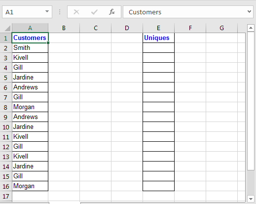
So here I have this list of customers in Column A in range A2:A16. Now in column E, I want to get unique values only from customers. Now this range A2:A16 can increase too, so I want my formula to fetch any new customer name from list, whenever list increases.

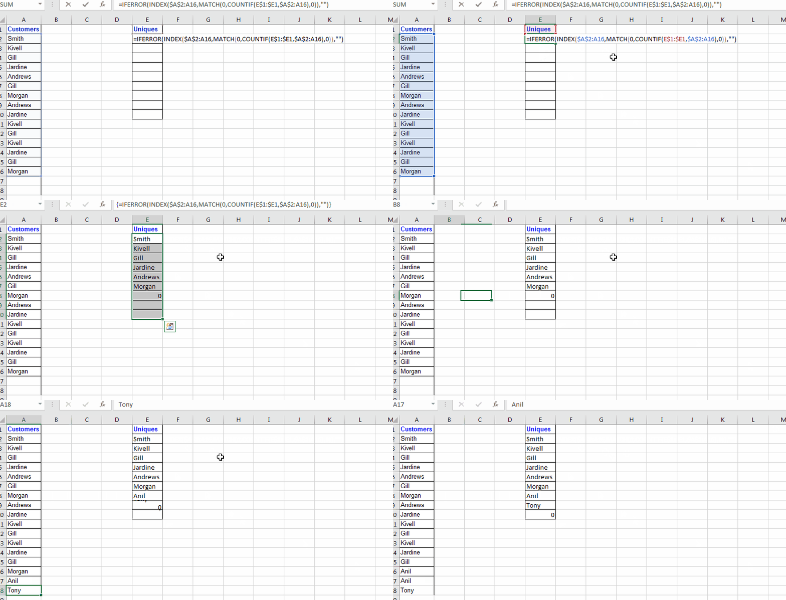
Ok, Now to fetch unique values from Column A write this formula in Cell E2, and hit CTRL+SHIFT+ENTER to make it an array formula.

A$2:A16: I expect that list will expand and may have new unique values that I will like to extract. That is why I have left it open from bottom by not absolute reference of A16. It will allow it to expand whenever you copy formula bellow.
So we know how INDEX and MATCH function works. The main part here is:
COUNTIF($E$1:E1,$A$2:A16): This formula will return an array of 1s and 0s. Whenever a value in range $E$1:E1 is found in criteria list $A$2:A16, the value converts into 1 at its position in the range $A$2:A16.
Now using MATCH function we are looking for values 0. Match will return position of first 0 found in array returned by COUNTIF function. Than INDEX will look into A$2:A16 to return value found at index returned by MATCH function.
It maybe a little bit hard to grasp but it works. The 0 in the end of the list indicates that there are no more unique values. If you don't see that 0 in the end you should copy the formula in below cells.
Now to avoid #NA in you can use IFERROR function of excel.
So yeah, you can use this formula to get unique values from a list. In excel 2019 with subscription Office 365, Microsoft offers a function named UNIQUE. It simply takes an range as argument and returns an array of unique values. Its not available in Microsoft Excel 2016 one time purchase.
Download file:
Related Articles:
Excel Formula to Extract Unique Values From a List
How to Count Unique Values In Excel
Popular Articles:
50 Excel Shortcuts to Increase Your Productivity
How to use the VLOOKUP Function in Excel
The applications/code on this site are distributed as is and without warranties or liability. In no event shall the owner of the copyrights, or the authors of the applications/code be liable for any loss of profit, any problems or any damage resulting from the use or evaluation of the applications/code.