How to use the MATCH function in Excel

In this article, we will learn How to use the MATCH function in Excel.

Why do we use the MATCH function ?

Given a table of 500 rows and 50 columns and we need to get a row index value at 455th row and 26th column. For this either we can scroll down to the 455th row and traverse to the 26th column and copy the value. But we can't treat Excel like hard copies. MATCH function returns the INDEX at a given row and column value in a table array. Let's learn the MATCH function Syntax and illustrate how to use the function in Excel below.

MATCH Function in Excel

The MATCH function in excel just returns the index of first appearance of a value in an array (single dimension). This function is mostly associated with the INDEX function, often known as the INDEX-MATCH function.

Syntax of MATCH Function:

=MATCH(lookup value, lookup array, match type)

lookup value : The value you are looking for in the array.

lookup array : The arrays in which you are looking for a value

Match Type : The match type. 0 for exact match, 1 for less than and -1 for greater than.

Example :

All of these might be confusing to understand. Let's understand how to use the function using an example.

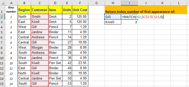
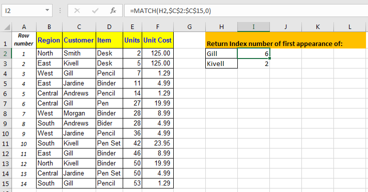
Here In the above image, we have a table. In cell H1, we have our task returning Index number of first appearance of Gill and Kivell.

In cell I2, write this formula and drag it down to I3.

=MATCH(H2,$C$2:$C$15,0)

We have our index numbers.

Now you can use this index number with INDEX function of excel to retrieve data from tables.

If you don’t know how to use INDEX MATCH function to retrieve data, below article will be helpful for you.

https://www.exceltip.com/lookup-formulas/retrieving-matching-values-from-not-adjacent-list.html

Do you know how to use the MATCH formula with VLOOKUP to automate reports? In Next article we will learn the use of VLOOKUP MATCH formula. Till then, Keep Practicing - Keep Excelling.

Use of INDEX & MATCH function to lookup value

Here we have a list of scores gained by students with their Subject list. We need to find the Score for a specific Student (Gary) & Subject (Social Studies) as shown in the snapshot below.

The Student value1 must match the Row_header array and Subject value2 must match the Column_header array.

Use the formula in the J6 cell:

= INDEX ( table , MATCH ( J5, row, 0 , MATCH ( J4, column, 0 ) ) )

Explanation:

The MATCH function matches the Student value in J4 cell with the row header array and returns its position 3 as a number.
The MATCH function matches the Subject value in J5 cell with the column header array and returns its position 4 as a number.
The INDEX function takes the row and column index number and looks up in the table data and returns the matched value.
The MATCH type argument is fixed to 0. As the formula will extract the exact match.

Here values to the formula is given as cell references and row_header, table and column_header given as named ranges.

As you can see in the above snapshot, we got the Score obtained by student Gary in Subject Social Studies as 36 . And it proves the formula works fine and for doubts see the below notes for understanding.

Now we will use the approximate match with row headers and column headers as numbers. Approx match only takes the number values as there is no way it applies on text values

Here we have a price of values as per the Height & Width of the product. We need to find the Price for a specific Height (34) & Width (21) as shown in the snapshot below.

The Height value1 must match the Row_header array and Width value2 must match the Column_header array.

Use the formula in the K6 cell:

= INDEX ( data , MATCH ( K4, Height, 1 , MATCH ( K5, Width, 1 ) ) )

Explanation:

The MATCH function matches the Height value in K4 cell with the row header array and returns its position 3 as a number.
The MATCH function matches the Width value in K5 cell with the column header array and returns its position 2 as a number.
The INDEX function takes the row and column index number and looks up in the table data and returns the matched value.
The MATCH type argument is fixed to 1. As the formula will extract the approximate match.

Here values to the formula is given as cell references and row_header, data and column_header given as named ranges as mentioned in the snapshot above.

As you can see in the above snapshot, we got the Price obtained by height (34) & Width (21) as 53.10 . And it proves the formula works fine and for doubts see the below notes for more understanding.

You can also perform lookup exact matches using INDEX and MATCH function in Excel. Learn more about How to do Case Sensitive Lookup using INDEX & MATCH function in Excel. You can also look up for the partial matches using the wildcards in Excel.

Notes:

The function returns the #NA error if the lookup array argument to the MATCH function is 2 D array which is the header field of the data..
The function matches the exact value as the match type argument to the MATCH function is 0.
The lookup values can be given as cell reference or directly using quote symbol ( " ) in the formula as arguments.

Hope this article about How to use the MATCH function in Excel is explanatory. Find more articles on finding values and related Excel formulas here. If you liked our blogs, share it with your friends on Facebook. And also you can follow us on Twitter and Facebook. We would love to hear from you, do let us know how we can improve, complement or innovate our work and make it better for you. Write to us at info@exceltip.com.

Related Articles :

Use INDEX and MATCH to Lookup Value : The INDEX & MATCH formula is used to lookup dynamically and precisely a value in a given table. This is an alternative to the VLOOKUP function and it overcomes the shortcomings of the VLOOKUP function.

Use VLOOKUP from Two or More Lookup Tables : To lookup from multiple tables we can take an IFERROR approach. To lookup from multiple tables, it takes the error as a switch for the next table. Another method can be an If approach.

How to do Case Sensitive Lookup in Excel : The excel's VLOOKUP function isn’t case sensitive and it will return the first matched value from the list. INDEX-MATCH is no exception but it can be modified to make it case sensitive.

Lookup Frequently Appearing Text with Criteria in Excel : The lookup most frequently appears in text in a range we use the INDEX-MATCH with MODE function.

Popular Articles :

How to use the IF Function in Excel : The IF statement in Excel checks the condition and returns a specific value if the condition is TRUE or returns another specific value if FALSE.

How to use the VLOOKUP Function in Excel : This is one of the most used and popular functions of excel that is used to lookup value from different ranges and sheets.

How to use the SUMIF Function in Excel : This is another dashboard essential function. This helps you sum up values on specific conditions.

How to use the COUNTIF Function in Excel : Count values with conditions using this amazing function. You don't need to filter your data to count specific values. Countif function is essential to prepare your dashboard.