In this article, we will learn how to Find nth smallest with criteria & nth largest with criteria from the given table in Excel.
Scenario:
In simple words, while working with numbers in data numbers, sometimes given a condition i.e. when we need to look up for the 5th highest value given . You can perform the solution to this problem easily using the excel functions as explained below.
Nth largest with criteria
How to solve the problem?
For this article we will be required to use the LARGE function. Now we will make a formula out of these functions. Here we are given a table and we need to find the nth largest value in range with given criteria.
Generic formula:
c_range : criteria range
value : criteria match value
range : result array
n : nth largest
Note : Do not put curly brackets manually. This is an array formula, must use Ctrl + Shift + Enter in place of just Enter where it returns #NUM! error.
Example:
All of these might be confusing to understand. So, let's test this formula via running it on the example shown below.
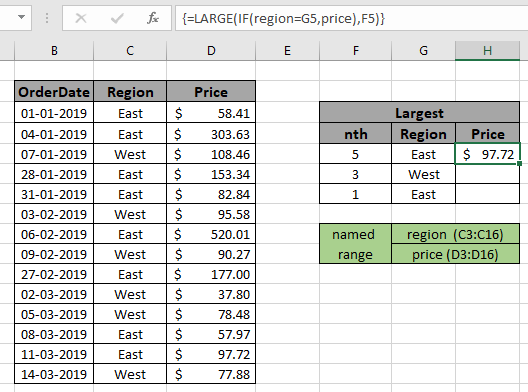
Here we have order details having date of order, region and order price.

We need to find out the 5th largest order price from East region. Here the range is given as using the named range excel tool.
region (C3:C16)
price (D3:D16)
Firstly, we need to find the Fifth largest values using the LARGE function and then sum operation be performed over those 5 values. Now we will use the following formula to get the sum
Use the Formula:
Explanation:
= LARGE ( { 58.41 ; 303.63 ; FALSE ; 153.34 ; 82.84 ; FALSE ; 520.01 ; FALSE ; 177 ; FALSE ; FALSE ; 57.97 ; 97.72 ; FALSE } ) , F5 )

You can view the formula in the formula box like as shown above snapshot. Use Ctrl + Shift + Enter to get the result.

As you can see the array formula returns the 5th largest price $97.72 having East region.
You can also feed array as array, criteria within quotes and n value directly to the function instead of using cell reference or named range.
Use the Formula:
Use Ctrl + Shift + Enter

You can see the formula works fine where find the nth largest value having criteria in table.
Nth lowest with criteria
How to solve the problem?
For this article we will be required to use the SMALL function. Now we will make a formula out of these functions. Here we are given a table and we need to find the nth smallest value in range with given criteria.
Generic formula:
c_range : criteria range
value : criteria match value
range : result array
n : nth largest
Note : Do not put curly brackets manually. This is an array formula, must use Ctrl + Shift + Enter in place of just Enter where it returns #NUM! error.
Example:
All of these might be confusing to understand. So, let's test this formula via running it on the example shown below.
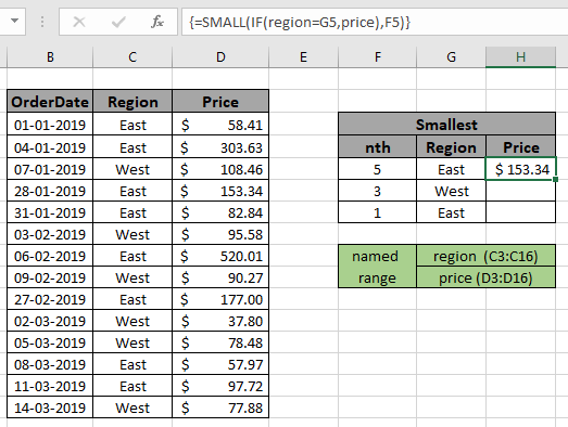
Here we have order details having date of order, region and order price.

We need to find out the nth smallest order price from East region. Here the range is given as using the named range excel tool.
region (C3:C16)
price (D3:D16)
Firstly, we need to find the Fifth smallest or lowest values using the SMALL function and then look up operation be performed over the values. Now we will use the following formula to get the sum
Use the Formula:
Explanation:
= LARGE ( { 58.41 ; 303.63 ; FALSE ; 153.34 ; 82.84 ; FALSE ; 520.01 ; FALSE ; 177 ; FALSE ; FALSE ; 57.97 ; 97.72 ; FALSE } ) , F5 )

You can view the formula in the formula box like as shown above snapshot. Use Ctrl + Shift + Enter to get the result.

As you can see the array formula returns the 5th smallest price $153.34 having East region.
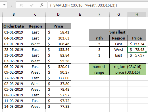
You can also feed array as array, criteria within quotes and n value directly to the function instead of using cell reference or named range.
Use the Formula:
Use Ctrl + Shift + Enter

You can see the formula works fine where you find the nth largest value having criteria in the table.
Here are some observational notes shown below.
Notes:
Hope this article about how to Find nth largest with criteria & nth smallest with criteria in excel is explanatory. Explore more articles on lookup formuls in Excel here. If you liked our blogs, share it with your friends on Facebook. And also you can follow us on Twitter and Facebook. We would love to hear from you, do let us know how we can improve, complement or innovate our work and make it better for you. Write us at info@exceltip.com
Related Articles
How to use the SUMPRODUCT function in Excel: Returns the SUM after multiplication of values in multiple arrays in excel.
SUM if date is between : Returns the SUM of values between given dates or period in excel.
Sum if date is greater than given date: Returns the SUM of values after the given date or period in excel.
2 Ways to Sum by Month in Excel: Returns the SUM of values within a given specific month in excel.
How to Sum Multiple Columns with Condition: Returns the SUM of values across multiple columns having condition in excel
How to use wildcards in excel : Count cells matching phrases using the wildcards in excel
Popular Articles
50 Excel Shortcut to Increase Your Productivity : Get faster at your task. These 50 shortcuts will make you work even faster on Excel.
How to use the VLOOKUP Function in Excel : This is one of the most used and popular functions of excel that is used to lookup value from different ranges and sheets.
How to use the COUNTIF function in Excel : Count values with conditions using this amazing function. You don't need to filter your data to count specific values. Countif function is essential to prepare your dashboard.
How to Use SUMIF Function in Excel : This is another dashboard essential function. This helps you sum up values on specific conditions.
The applications/code on this site are distributed as is and without warranties or liability. In no event shall the owner of the copyrights, or the authors of the applications/code be liable for any loss of profit, any problems or any damage resulting from the use or evaluation of the applications/code.