Finding Every Third Number and Returning the Largest of Them in Microsoft Excel 2010

If you want to find the largest every third number in a list of numbers, we can use the combination of IF, MAX, MOD & ROW functions.

The "IF function" checks if a condition you specify is TRUE or FALSE. If the condition returns TRUE then it returns preset value, if the condition returns FALSE then it returns another preset value.

Syntax = IF(logical_test,value_if_true,value_if_false)

logical_test: Logical test will test the condition or criteria, if condition meets then it returns the preset value, and if condition does not meet then it returns another preset value.

value_if_true: The value that you want to be returned if this argument returns TRUE.

value_if_false: The value that you want to be returned if this argument returns FALSE

"MAX": Returns the maximum

number from a range of cells or array. For example,if a list of numbers contains 5, 6, 7, 8, 9 & 10, then the output will be 10.

Syntax =MAX(number1,number2,...)

number1:These are numeric values.They can be numbers, named ranges or arrays. The first value argument represents the values that you have taken as a reference.

number2:These are numeric values.They can be numbers, name ranges or arrays. The second value argument represents the values that you have taken as a reference.

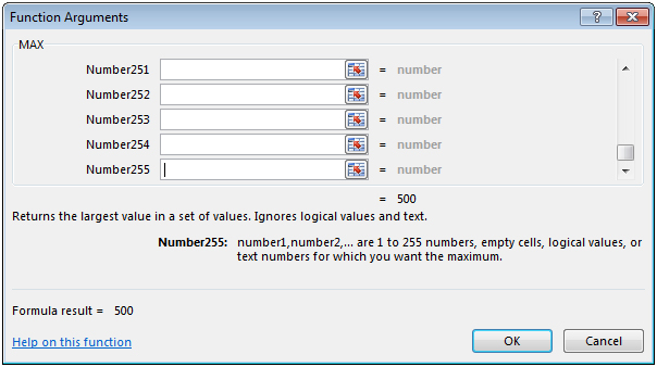
There can be a maximum of 255 arguments.Refer the below shown screenshot:

"MOD": Returns the remainder after a number is divided by a divisor.

Syntax =MOD(number,divisor)

number: It is a numeric value whose remainder you want to find.

divisor: It is the number which is used to divide the number argument.

"ROW": Returns the row number of a reference.

Syntax: =ROW(reference)

Reference: It is a reference to a cell or range of cells.

Let us take an example:

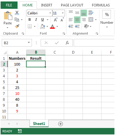
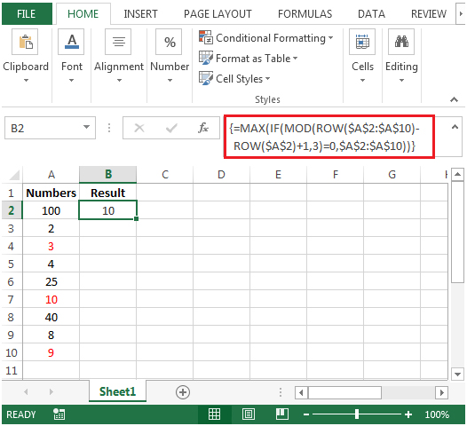
We have some random numbers in column A. We need a formula in cell B2 to look for each set of 3 numbers from a list in column A &find the largest number for this set. Every third number is highlighted in red.

• In cell B2, the formula would be
• =MAX(IF(MOD(ROW($A$2:$A$10)-ROW($A$2)+1,3)=0,$A$2:$A$10))
• This is an array formula, we press CTRL + SHIFT + ENTER, formula will be enclosed with curly brackets by using this.
• {=MAX(IF(MOD(ROW($A$2:$A$10)-ROW($A$2)+1,3)=0,$A$2:$A$10))}

• The output we get is 10, although there are numbers greater than 10. This is because the above mentioned formula is checking every third number in the range.If it is the highest out of all, the formula ignores values which are at 1^st& 2^ndposition in the range. In our example, 100 & 2 are the 1^st& 2^ndnumbers.
• The formula checks cells A2:A4 and finds that the 3^rd number is 3. In range A5:A7, the 3^rd number is 10 and in the range A8:A10, the 3^rd number is 9. The largest number from these 3 numbers (3,10,9) is 10. Hence the output is 10.