Normally, the VLOOKUP function returns the first match it finds. But the matter gets complicated when there more than one match and we want to get any specific occurrence, say 2nd match.
In this article, we will learn how to get second, third or Nth match using VLOOKUP. To achieve this we will need to use a helper column. If you don't want to use a helper column as it is not feasible with every data, you can use the INDEX-MATCH approach. But if you can use a helper column, here's the generic formula to find Nth match using VLOOKUP Function.
| =VLOOKUP(lookup_value&occurrence,table_array,column,0) |
Lookup_value: It is the lookup value that you want to look for.
Occurrence: The occurrence of lookup value that you want to match.
Table_array: It is the table array in which you want to look for data. Make sure that the first column in this table is the helper column.
Column: The column number in the table array from which you want to retrieve the value.
0: It is for an exact match. If you don't want to do an exact match, omit it or use 1 or TRUE.
Now let's use it in an example:

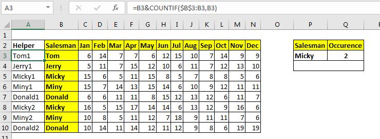
We have a table that records sales done by salesmen in different months. The names of the salesmen can repeat in the record. We need to match the 2nd occurrence of Micky and then get Jan's sales.
Note that, we have added a helper column. This column writes the name of the salesman and then concatenates the occurrence of that name to it. We have used the running count to get the occurrence.
The formula in helper column is:
| =B3&COUNTIF($B$3:B3,B3) |
So, we have the table ready. Here the lookup value is in cell P3, the occurrence number is in Q3, the table array is A3:N10 and the column number is 3.
Now write this formula in cell P4:
| =VLOOKUP(P3&Q3,A3:N10,3,0) |
Hit enter, and bam! you have your lookup value of the occurrence you needed.

How does it work?
The functionality is simple. Initially, we don't have any unique id to use as a lookup value. So we create one. We use the name and running count formula to create a unique ID. We make sure that it is first column in the table from left as we are going to use to retrieve values from columns right to it.
Now the lookup formula creates the unique id using concatenate operator & ( P3&Q3). This makes it a unique Id
Next, the VLOOKUP formula takes this as lookup value and looks for its location in table A3:N10. Here, VLOOKUP finds the value in 6th row of the table. Now it moves to the 3rd column and returns the value.
This is the easiest way to get the Nth match in Excel. But it is not feasible all the time. It adds extra data and calculations to the sheet that can make the excel file heavy and slow.
If you have a small amount of data, this is great but with large data, you may want to use an independent formula that does not need helper column. In that case, you can use an array formula that uses INDEX and MATCH functions.
So yeah guys, this how you can get the Nth match in Excel using VLOOKUP function. I hope I was explanatory enough and it was helpful. If you have any doubts regarding this article or any other excel/VBA related topic, ask in the comments section below.
Related Articles:
Lookup nth match using INDEX & MATCH function | To get nth match without using a helper column we use INDEX and MATCH function. We use the boolean logic to get the index from the table.
How to LOOKUP Multiple Values | To retrieve all the matching values from a list, we use the INDEX MATCH function. VLOOKUP can retrieve multiple values only when we use a helper column.
Lookup Value with Multiple Criteria | If you have to lookup more than one lookup tables then how do you use VLOOKUP from two Lookup tables or more. This article solves this problem very easily
Lookup Value with Multiple Criteria | We can simply use the VLOOKUP function. But when you don’t have that unique column in your data and need to lookup in multiple columns to match a value, VLOOKUP doesn’t help
How To Look Up Address in Excel | There will be times when you would want to get the address of the cell from which a value is being retrieved. Using that address you can easily retrieve adjacent values using the OFFSET function
Popular Articles:
50 Excel Shortcuts to Increase Your Productivity | Get faster at your task. These 50 shortcuts will make you work even faster on Excel.
How to use Excel VLOOKUP Function| This is one of the most used and popular functions of excel that is used to lookup value from different ranges and sheets.
How to use the Excel COUNTIF Function| Count values with conditions using this amazing function. You don't need to filter your data to count specific value. Countif function is essential to prepare your dashboard.
How to Use SUMIF Function in Excel | This is another dashboard essential function. This helps you sum up values on specific conditions.
The applications/code on this site are distributed as is and without warranties or liability. In no event shall the owner of the copyrights, or the authors of the applications/code be liable for any loss of profit, any problems or any damage resulting from the use or evaluation of the applications/code.