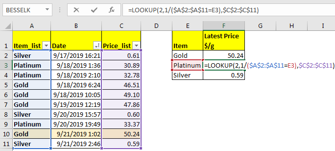
Let’s say you maintain data of different items in a list. The latest price of an item can be found by looking last entry of that item. So, if your data is sorted oldest to newest, we just need the formula to retrieve the last entry of an item and then look at its price. We can do this using Excel LOOKUP function.
Generic Formula
Item_list: This is the list of items. Basically a one-dimensional range also called vector.
Item : The item for which we are looking for.
Price_list: This the price list corresponding to items in item_list. This also a vector.
Let’s learn by example.
Example: Fetch the Latest Price of Valuable Metals in Excel
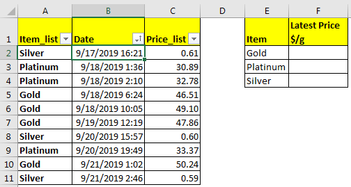
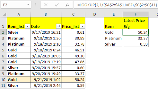
Here we have a list of item and their price. The list is sorted oldest to newest using date and time column. I have kept this list small so that it gets easy to explain.

Range A2:A11 is our Item_list and range C2:C11 is price_list. Column B contains date and time. We have sorted the table using date column.
In E column, we have list of unique items. In Column F we need to retrieve the latest price of these items from table.
Write this formula in cell F2:
This will retrieve the latest price of gold in list. To copy it in below cells make it generic.
Here I have used absolute references for lists so that they don’t change when copied down.

How it works:
It works on the method of retrieving last matched value. So, the LOOKUP function returns last value found that was less than lookup value. We use this feature to get latest price of an item in the list.
Let’s brack down the formula.
(A2:A11="gold"): This statement returns an array of TRUE and FALSE. TRUE if cell in A2:A11 contains “gold” else FALSE. {FALSE;FALSE;FALSE;TRUE;TRUE;TRUE;FALSE;FALSE;TRUE;FALSE}.
1/(item_list= “item”): Next, we divide 1 by this array. This gives us an array 1 and #DIV/0 errors.
{#DIV/0!;#DIV/0!;#DIV/0!;1;1;1;#DIV/0!;#DIV/0!;1;#DIV/0!}.
LOOKUP(2,{#DIV/0!;#DIV/0!;#DIV/0!;1;1;1;#DIV/0!;#DIV/0!;1;#DIV/0!}),$C$2:$C$11) : Now formula is this. LOOKUP looks for 2 in array. Since the maximum value is 1 here, LOOKUP returns last 1 according to its property, which is at 9th position in array. Lookup looks at 9th position in result vector $C$2:$C$11 and returns the value, which is 50.24 here.
Download file:
Related Articles:
Use INDEX and MATCH to Lookup Value in Excel
How to use the LOOKUP function in Excel
Lookup Value with Multiple Criteria in Excel
Popular Articles
50 Excel Shortcut to Increase Your Productivity: Get faster at your task. These 50 shortcuts will make you work even faster on Excel.
How to use the VLOOKUP Function in Excel: This is one of the most used and popular functions of excel that is used to lookup value from different ranges and sheets.
How to use the COUNTIF function in Excel: Count values with conditions using this amazing function. You don't need to filter your data to count specific values. Countif function is essential to prepare your dashboard.
How to use the SUMIF Function in Excel: This is another dashboard essential function. This helps you sum up values on specific conditions.
The applications/code on this site are distributed as is and without warranties or liability. In no event shall the owner of the copyrights, or the authors of the applications/code be liable for any loss of profit, any problems or any damage resulting from the use or evaluation of the applications/code.