In this article, we will learn How to look up or find value with last Date in Excel.
Lookup a value and find max or last date
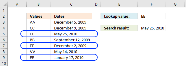
The picture below shows you values in column B (B3:B9) and dates in column C (C3:C9). The formula in cell F4 lets you search for value and return the latest date in an adjacent or corresponding column for that value.

Update, 2017-08-15! Added a regular formula.
Formula in cell F4:
| =MAX(INDEX((C3=A8:A14)*B8:B14,)) |
Array formula in F4:
| =MAX(IF(C3=A8:A14, B8:B14)) |
Formula in cell F4 (Excel newer versions):
| =MAXIFS(C3:C9,B3:B9,F2) |
How to create an array formula
The formula changes and now begins and ends with a curly bracket, don't enter these characters yourself. They appear automatically.
Explaining array formula in cell C5
You can follow along if you select cell C5 and go to tab "Formulas" on the ribbon and then click the "Evaluate Formula" button. Click the "Evaluate" button, shown on the dialog box, to move to the next step.
Step 1 - Find values equal to lookup value
C3=A8:A14
becomes
"EE"={"AA";"CC";"EE";"BB";"EE";"VV";"EE"}
and returns
{FALSE;FALSE;TRUE;FALSE;TRUE;FALSE;TRUE}
Step 2 - Convert boolean values to corresponding dates
IF(C3=A8:A14, B8:B14)
becomes
IF({FALSE;FALSE;TRUE;FALSE;TRUE;FALSE;TRUE} ,B8:B14)
becomes
IF({FALSE;FALSE;TRUE;FALSE;TRUE;FALSE;TRUE} , {40152; 40156; 40323; 40068; 40149; 40312; 40195})
and returns
{FALSE;FALSE;40323;FALSE;40149;FALSE;40195}
Step 3 - Return the largest value
=MAX(IF(C3=A8:A14, B8:B14))
becomes
=MAX({FALSE;FALSE;40323;FALSE;40149;FALSE;40195})
and returns 40323 formatted as 2010-05-25.
Lookup a value and find max date (Pivot Table)

The formulas demonstrated in this article may be too slow or take too much memory if you work with huge amounts of data. The Pivot Table is an excellent option in such cases, it is remarkably fast even with lots of data.
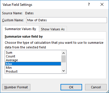
How to set up Pivot Table


I usually place the Pivot Table on a new worksheet so it doesn't hide parts of the data set while filtering etc.


Click on cell B1 to filter the latest date based on the selected value, the image above shows value EE selected and the latest date based on that value is 5/25/2010.
Lookup all values and find latest (earliest) date
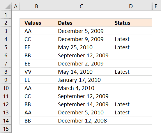
The following formula looks in column C for the most recent date for each value in column B.

Formula in cell D3:
| =IF(MAX(INDEX((B3=$B$3:$B$14)*$C$3:$C$14,))=C3,"Latest","") |
Array formula in cell D3:
| =IF(MAX(IF(B3=$B$3:$B$14, $C$3:$C$14))=C3, "Latest", "") |
Formula in cell D3:
| =IF(MAXIFS($C$3:$C$14,$B$3:$B$14,B3)=C3,"Latest","") |
How to copy array formula
Lookup and find last date using multiple conditions

Formula in cell H3:
| =MAX(INDEX((C2:C29=H1)*(D2:D29=H2)*E2:E29,)) |
Array formula in cell H3:
| =MAX(IF((C2:C29=H1)*(D2:D29=H2),E2:E29,"")) |
Lookup and find latest date on multiple sheets
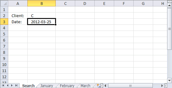
The following picture shows you a workbook with 4 worksheets. The formula in cell B3 looks for the latest date in all three worksheets using the condition in cell B2.

Array formula in cell B3:
| =MAX(IF(B2=January!$B$2:$B$10, January!$A$2:$A$10, ""), IF(B2=February!$B$2:$B$10, February!$A$2:$A$10, ""), IF(B2=March!$B$2:$B$10, March!$A$2:$A$10, "")) |
Lookup and find latest date, return corresponding value on same row

Enter a quarter in cell G3.
Array formula in cell G3:
| =MAX((B3:B19=G2)*C3:C19) |
If you prefer a regular formula in G3:
=MAX(INDEX((B3:B19=G2)*C3:C19,))
Formula in cell G4:
| =INDEX($D$3:$D$19, SUMPRODUCT((B3:B19=G2)*(G3=C3:C19)*MATCH(ROW(B3:B19), ROW(B3:B19)))) |
Index & Match to Find Value by Latest Date in Microsoft Excel
If you are looking for a formula to find the lookup value & latest value by date, then this article is really helpful for you. In this article, we will learn how to find the matching value & then formula will check the output after checking the latest date.
Example: I need a formula to look up each specific product then find the price of the product on the latest date.
Following is the snapshot of data i.e. column A has Invoice No., column B has Date, column C has Product & column D has Prices.
The formula we are looking for should first of all check the Product from column C & then return the Price for the latest date.
We will use a combination of INDEX, MATCH & MAX functions to return the output.
In cell G3, the formula is
| {=INDEX($D$2:$D$10,MATCH(1,INDEX(($C$2:$C$10=$F$3)*($B$2:$B$10=MAX(IF($C$2:$C$10=F3,$B$2:$B$10))),0),0))} |
The above formula has used Max function to determine the latest date from all the given dates for the matching Product from column C. To test the above formula if we change the date in cell B7, then we will get the desired result. Refer below snapshot. In this way, we can deliver the price of the product with the latest date.
Here are all the observational notes using the formula in Excel
Notes :
This is an array formula. Hence, we need to press CTRL + SHIFT + END keys together to get the correct result.
Hope this article about How to lookup or find value with last Date in Excel is explanatory. Find more articles on calculating values and related Excel formulas here. If you liked our blogs, share them with your friends on Facebook. And also you can follow us on Twitter and Facebook. We would love to hear from you, do let us know how we can improve, complement or innovate our work and make it better for you. Write to us at info@exceltip.com.
Related Articles :
How to Retrieve Latest Price in Excel : It is common to update prices in any business and using the latest prices for any purchase or sales is a must. To retrieve the latest price from a list in Excel we use the LOOKUP function. The LOOKUP function fetches the latest price.
VLOOKUP function to calculate grade in Excel : To calculate grades IF and IFS are not the only functions that you can use. The VLOOKUP is more efficient and dynamic for such conditional calculations.To calculate grades using VLOOKUP we can use this formula.
17 Things About Excel VLOOKUP : VLOOKUP is most commonly used for retrieving matched values but VLOOKUP can do a lot more than this. Here are 17 things about VLOOKUP that you should know to use effectively.
LOOKUP the First Text from a List in Excel : The VLOOKUP function works fine with wildcard characters. We can use this to extract the first text value from a given list in excel. Here is the generic formula.
LOOKUP date with last value in list : To retrieve the date that contains the last value we use the LOOKUP function. This function checks for the cell that contains the last value in a vector and then uses that reference to return the date.
Popular Articles :
50 Excel Shortcuts to Increase Your Productivity : Get faster at your tasks in Excel. These shortcuts will help you increase your work efficiency in Excel.
How to use the VLOOKUP Function in Excel : This is one of the most used and popular functions of excel that is used to lookup value from different ranges and sheets.
How to use the IF Function in Excel : The IF statement in Excel checks the condition and returns a specific value if the condition is TRUE or returns another specific value if FALSE.
How to use the SUMIF Function in Excel : This is another dashboard essential function. This helps you sum up values on specific conditions.
How to use the COUNTIF Function in Excel : Count values with conditions using this amazing function. You don't need to filter your data to count specific values. Countif function is essential to prepare your dashboard.
The applications/code on this site are distributed as is and without warranties or liability. In no event shall the owner of the copyrights, or the authors of the applications/code be liable for any loss of profit, any problems or any damage resulting from the use or evaluation of the applications/code.
How to use name to find max or latest date in another sheet?
Use the sheet name before the range. let's say you want to find in sheet 1 then use this formula.
{=INDEX(Sheet1!$D$2:$D$10,MATCH(1,INDEX((Sheet1!$C$2:$C$10=$F$3)*(Sheet1!$B$2:$B$10=MAX(IF(Sheet1!$C$2:$C$10=F3,Sheet1!$B$2:$B$10))),0),0))}
Thank you very MUCH!!!!!!!!! Help me a lot!!!
What simple explanation!!!!!!