Lookup lowest match using INDEX & MATCH function

In this article, we will learn how to Lookup the lowest match using INDEX & MATCH function in Excel.

Scenario:

For instance, We need to find the numerically lowest match and its corresponding results from the table. We need some fixed formula which helps in finding the lowest match as to get the required value.

How to Solve the Problem?

For the formula to understand first we need to revise a little about the following functions

Now we will make a formula using the above functions. MATCH function will return the index of the lowest match from the range. The INDEX function takes the row index as argument and returns its corresponding required results.

Generic Formula:

= INDEX ( data , MATCH ( MIN (range), range, match_type ) , col_num )

data : array of values in the table without headers

range : lookup_array for the lowest match

match_type : 1 ( exact or next smallest ) or 0 ( exact match) or -1 ( exact or next largest )

col_num : column number, required value to retrieve from the table column.

Example:

The above statements can be complicated to understand. So let’s understand this by using the formula in an example

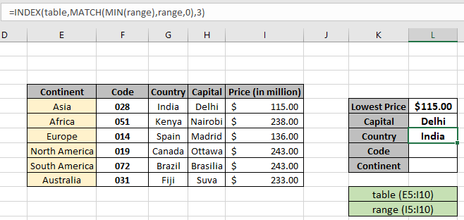
Here we have a table having details about the world continent. We need to find the country code from the given table from the lookup value as country name.

Named range used for table (E5:I10) & range (I5:I10) array.
Here we used the named range instead for cell reference array as it's easy to understand. We need to look for all the details where Price value is minimum or lowest in the range.

Use the above formula to get the first detail which is capital
Use the formula in the G6 cell:

= INDEX ( table , MATCH ( MIN (range) , range , 0 ) , 4 )

Named ranges

table (E5:I10)

range (I5:I10)

Explanation:

MATCH function matches the exact minimum value match in the Price range and returns its row index to the INDEX function.
The INDEX function finds the Capital value having ROW index and 4th column in the table named range.

The formula returns capital city for the minimum value. Now copy the formula using the Ctrl + D or drag down the cell option in excel. Just have to change the col_num argument to get the different details.

To extract code & Continent name from the formula use the formula to get code:

= INDEX ( table , MATCH ( MIN (range) , range , 0 ) , 2 )

To get the Continent value:

= INDEX ( table , MATCH ( MIN (range) , range , 0 ) , 1 )

As you can see from the above snapshot we obtained all the details matching minimum value in the table. Extract details from the table using the above stated formula.

Here are some observational noter while using the above formula.

Notes:

The function returns the #NA error if the lookup array argument to the MATCH function is not of same length of the table array.
The formula returns an error if lookup_value doesn't match the value in the table lookup_array.
The function matches exact value as the match type argument to the MATCH function is 0.
The lookup values can be given as cell reference or directly using quote symbol ( " ) in the formula as arguments.

Hope you understood how to Lookup lowest match using the INDEX & MATCH function in excel. Explore more articles on Excel lookup value here. Please feel free to state your queries below in the comment box. We will certainly help you.

If you liked our blogs, share it with your friends on Facebook. And also you can follow us on Twitter and Facebook. We would love to hear from you, do let us know how we can improve, complement or innovate our work and make it better for you. Write us at info@exceltip.com

Related Articles

Use INDEX and MATCH to Lookup Value : INDEX & MATCH function to look up value as required.
SUM range with INDEX in Excel : Use INDEX function to find the SUM of the values as required.
How to use the INDEX function in Excel : Find the INDEX of array using the INDEX function explained with example.
How to use the MATCH function in Excel : Find the MATCH in the array using the INDEX value inside MATCH function explained with example.
How to use LOOKUP function in Excel : Find the lookup value in the array using the LOOKUP function explained with example.
How to use the VLOOKUP function in Excel : Find the lookup value in the array using the VLOOKUP function explained with example.