Since you are here, I assume that you want to look up some values in multiple tables. If any of the tables contains the given lookup value, you want to retrieve them using Excel VLOOKUP function. Right? Here's how you do it.
Generic Formula for the nested VLOOKUP function
| =IFERROR(VLOOKUP(lookup_value,table1,col,0),IFERROR(VLOOKUP(lookup_value,table2,col,0),VLOOKUP(lookup_value,table3,col,0))) |
lookup_value: This the value you are looking for in your record.
Table1, Tabl2, Table3,...: These are the tables in which you know that the value exists.
col: The column number in the table from which you want to fetch the value.
0: This is for an exact match. If you want to do an approximate match use 1.
Let's have an example make things clear.
Using nested VLOOKUPs to search multiple tables
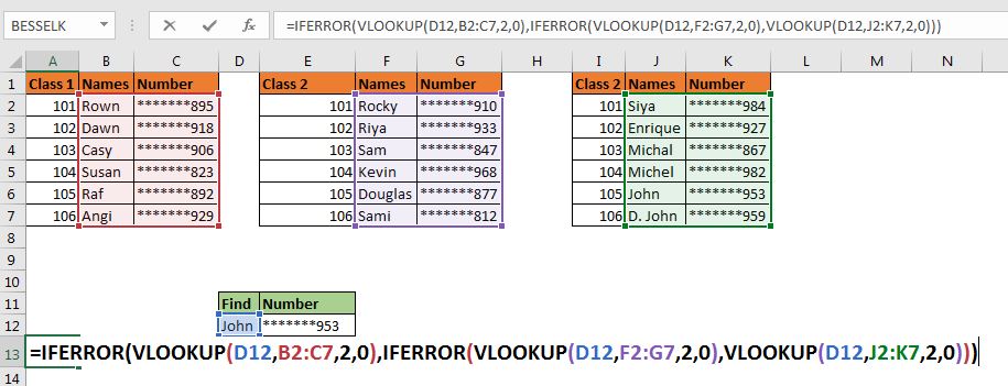
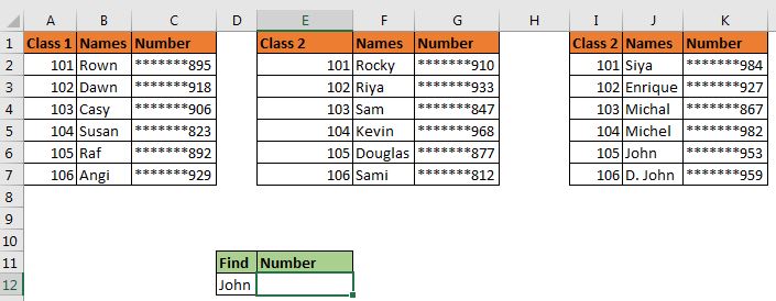
Let's create a scenario first. Assume that we run three Yoga classes. At the end of the day, you find a wrist band that has the name John on it. Now you know that John belongs to one of three classes. To lookup john in all three classes, we will need to put nested or chained VLOOKUP function inside the IFERROR functions.

Here, we want to lookup john using VLOOKUP in all three tables and fetch his phone number.
Using the above generic formula, we put this formula in cell E12.
| =IFERROR(VLOOKUP(D12,B2:C7,2,0),IFERROR(VLOOKUP(D12,F2:G7,2,0),VLOOKUP(D12,J2:K7,2,0))) |
Here, D12 is our lookup value.
B2:C7, F2:G7, and J2:K7 are the tables that we want to search in.
2 is the column number of tables from which we want to retrieve the number. (Here column number is the same for every table, but it can be different in different data sets).
When you hit the enter button, it retrieves john's number.

How does it work
The technique is simple. As we know that VLOOKUP throws #N/A error when it fails to find the lookup value in the given table, and IFERROR function returns specified value if it fed an #N/A error. We use these features in our advantage.
The first VLOOKUP runs. It fails to find John in the first table. It returns #N/A error. Now, this function is encapsulated in the IFERROR function. Since the first VLOOKUP formula has fed #N/A to IFERROR, the second part of IFERROR runs, which again contains an IFERROR function.
In the next round, the VLOOKUP looks for john in the second table F2:G7. It fails again and IFERROR bounces the control to the next part. In this part, we only have VLOOKUP Function but this time it finds john in the third table J2:K7 and returns the number.
Note: In the above example, we were sure that John is part of one three tables. But if you are not sure that your tables contain these values or not then use another IFERROR function that tells return "Value not found in any table".
| =IFERROR(VLOOKUP(D12,B2:C7,2,0),IFERROR(VLOOKUP(D12,F2:G7,2,0),IFERROR(VLOOKUP(D12,J2:K7,2,0),"Can't find"))) |
So yeah guys, this how you can look up into multiple tables. This is not the most elegant way to lookup multiple tables but this is what we have. There are other ways of doing it. One way is to haveing a combined data set of all classes in one master file. Another is always VBA.
I hope I was explanatory enough. If you have any doubts regarding this article or any other excel or VBA related article, let me know in the comments section below.
Related Articles:
IFERROR and VLOOKUP function | The VLOOKUP function is itself an amazing function but works even better when used with the IFERROR function. The IFERROR function is used to catch any error returned by the VLOOKUP function.
ISERROR and VLOOKUP function | This combination returns TRUE if the VLOOKUP function results in an error.
17 Things About Excel VLOOKUP | Learn 17 amazing features of VLOOKUP in one go.
LOOKUP Multiple Values | Lookup Multiple matches using the INDEX-MATCH function.
Popular Articles:
50 Excel Shortcuts to Increase Your Productivity | Get faster at your task. These 50 shortcuts will make you work even faster on Excel.
The VLOOKUP Function in Excel | This is one of the most used and popular functions of excel that is used to lookup value from different ranges and sheets.
COUNTIF in Excel 2016 | Count values with conditions using this amazing function. You don't need filter your data to count specific value. Countif function is essential to prepare your dashboard.
How to Use SUMIF Function in Excel | This is another dashboard essential function. This helps you sum up values on specific conditions.
The applications/code on this site are distributed as is and without warranties or liability. In no event shall the owner of the copyrights, or the authors of the applications/code be liable for any loss of profit, any problems or any damage resulting from the use or evaluation of the applications/code.