In this article, we will learn how to use ISERROR function along with the VLOOKUP function to ignore the error as result in Microsoft Excel.
Considering we have this situation where we want to create a formula to check for each successful search. The formula should return that number, when the match is found. And, if an exact match is not found, the formula should return a text message to that effect, rather than an error in Microsoft Excel.
If it is error in Excel Vlookup formula, we will use IF, Iserror and Vlookup function to prevent the #N/A error.
VLOOKUP is an Excel function which is used to lookup and retrieve data from a specific column of a table. Lookup values must appear in the first column of the table, with lookup columns to the right.
Syntax:
| =VLOOKUP(lookup_value, table_array, col_index_num, [range_lookup]) |
ISERROR function used for checking the error while calculation by using any function. We use this function when excel vlookup not working or showing an error.
Syntax:
| =ISERROR(Formula) |
IF function works on logic_test and returns values based on the result of the test.
Syntax:
| =IF(Logic_test, [Value_if_True], [Value_if_False]) |
Let’s take an example to understand how we can prevent a Vlookup function from returning an error when an exact match is not found.
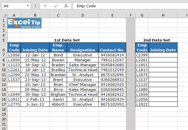
Here we have two tables named 1st Data set and 2nd Dat set.

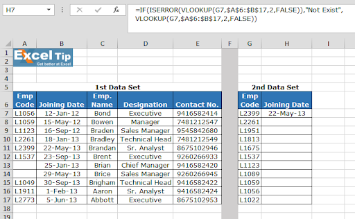
Write the VLOOKUP formula in H7 cell.
| =IF(ISNA(VLOOKUP(G3,$A$2:$B$13,2,FALSE)),”Number Not Found”, VLOOKUP(G3,$A$2:$B$13,2,FALSE)) |
Explanation:
Vlookup function checks the condition for the 2nd column of the 1st Data set matching EMP CODE in 1st Data set.
ISERROR function looks for any error and passes it on to the IF function.
IF function checks if an error occurs, it print “Not Exist” instead of the error.

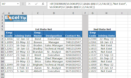
Copy the formula in other cells, select the cells taking the first cell where the formula is already applied, use shortcut key Ctrl + D.

As you can see in the above image that formula is working fine. And the user can work without getting irritated by any error. If ISERROR function is not used, vlookup returning n/a error is the output.
Hope you will use the VLOOKUP function. You can use the same functions in Excel 2016, 2013 and 2010. There are more articles on VLOOKUP and HLOOKUP. Please do check more links here and if you have any unresolved query, please state that in the comment box below. We will help you.
Related Articles:
How to use IF, ISNA and VLOOKUP function in Excel?
Partial match with VLOOKUP function
The applications/code on this site are distributed as is and without warranties or liability. In no event shall the owner of the copyrights, or the authors of the applications/code be liable for any loss of profit, any problems or any damage resulting from the use or evaluation of the applications/code.
WONDERFUL
Hi Sadeq,
Thanks a lot for the appreciation. 🙂
Happy Learning,
Site Admin
can you please explain the below formula -->
=IF(ISERROR(VLOOKUP($B18,'Profit Projections'!$A$11:$AB$110,'Profit Projections'!$AB$2,FALSE)),0,VLOOKUP($B18,'Profit Projections'!$A$11:$AB$110,'Profit Projections'!$AB$2,FALSE))
questions--
what is the formula trying to do?
why is the range defined twice ?