In this article we will learn how to find a value from a reference grid while using indexes list, we can use a combination of "OFFSET" & "MATCH" functions to get the output in Microsoft Excel 2010.
OFFSET: Returns areference to a range that is a given number of rows and columns from a given reference.
Syntax: =OFFSET(reference,rows,cols,height,width)
reference: It is a reference to a cell or range of cells from which the offset will be applied.
rows: The number of rows up or down that you want to apply as the offset to the range.
cols: The number of columns left or right that you want to apply as the offset to the range.
height: This is optional. It is the number of rows that you want the returned reference to be.
width: This is optional. It is the number of columns that you want the returned reference to be.
MATCH function searches for a specified item in a selected range of cells, and then returns the relative position of that item in the range.
Syntax =MATCH(lookup_value,lookup_array,match_type)
lookup_value: The value you want to look for
lookup_array: The table of data contains information from which you want to return the output.
match_type: 1,0 and -1 are three options.
1(Default): It will find the largest value in the range. List must be sorted in ascending order.
0: It will find an exact match
-1: It will find the smallest value in the range. List must be sorted in descending order.
Let us take an example:
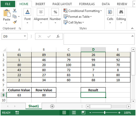
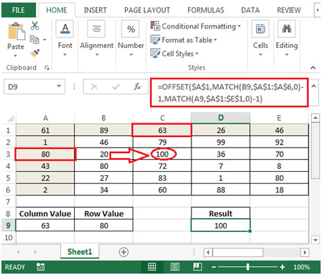
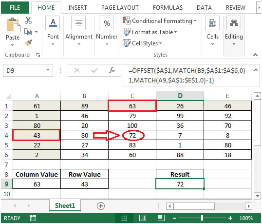
We have a list of some random numbers in range A1:E6.Cell A9 contains value from column range i.e. A1:E1. Cell B9 contains value from row range i.e. A1:A6. We need a formula to find the matching value from both column & row.


The applications/code on this site are distributed as is and without warranties or liability. In no event shall the owner of the copyrights, or the authors of the applications/code be liable for any loss of profit, any problems or any damage resulting from the use or evaluation of the applications/code.