How to use Index Match function in multiple criteria

In this article we will learn how to retrieve an item from a list that meets multiple criteria, we use Index and Match function in Microsoft Excel.

MATCH: The Match formula returns the cell number where the value is found in a horizontal or vertical range.

Syntax of “MATCH” function:=MATCH(lookup_value,lookup_array,[match_type])

There is 3 match type 1^st is 1-less than, 2^nd is 0-Exact match, 3^rd is (-1)-greater than. For example:- We have data in range A1: C5. Column A contains Order Id, column B contains Unit Price, and column C contains Quantity. Follow below given steps:-

Write the formula in cell D2.
=MATCH(12982,A2:A5,1), press Enter on your keyboard.
The function will return 4. It means 4^thcell is matching as per given criteria.

INDEX: The Index formula returns a value from the intersection between the row number and the column number in an Array. There are 2 syntaxes for the “INDEX” function.

1stSyntaxof“INDEX”function: =INDEX (array, row_num, [column_num])

2nd Syntax of “INDEX” function:=INDEX (reference, row_num, [column_num], [area_num])

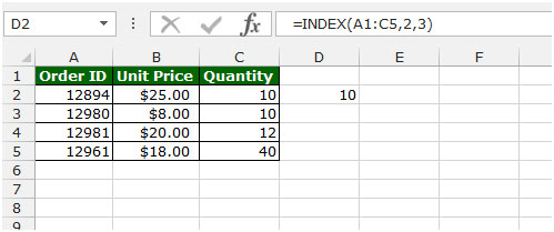
For example: - We have data in range A1:C5. Column A contains Order Id, column B contains Unit Price, and column C contains Quantity. Follow below given steps:-

Write the formula in cell D2.
=INDEX(A1:C5,2,3) press Enter on your keyboard.
The function will return 10. It means 10 is available in 2^nd row and 3^rd column.

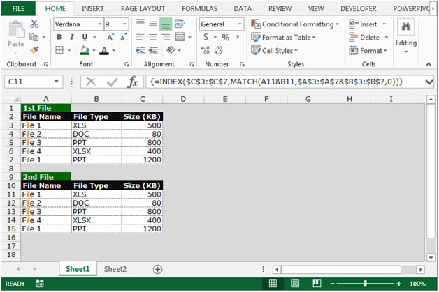
Let’s take an example to understand how to retrieve an item from a list that meets multiple criteria. We have 2 data sets. Range 1 (A2:C7) contains file names with their matching types and sizes. Range 2 (A10:B15) contains a similar list of file names but with matching types only. Now, we want to find the appropriate file sizes from Range1 by matching each pair of file names and types from both the ranges. Follow below given steps:-

Write the formula in cell C11.
=INDEX($C$3:$C$7,MATCH(A11&B11,$A$3:$A$7&$B$3:$B$7,0))
Press Ctrl+Shift+Enter on your keyboard to create an array formula.
{=INDEX($C$3:$C$7,MATCH(A11&B11,$A$3:$A$7&$B$3:$B$7,0))}
The function will return the file size after checking the multiple criteria.
Copy the same formula and paste one by one in each cell.

This is the way we can retrieve the item from a list that meets multiple criteria by using the Index function along with Match function in Microsoft Excel.

Tom Hasler
March 20, 2015 at 2:32 pm

I really appreciate this post. I'm attempting to create a formula where I'm matching two different criteria and returning a value. The one criteria is a SKU number and the other is a tier of values based on the quantity of a particular SKU. Here's the formula I'm using, but it's not returning the correct value. {=INDEX($P$2:$P$1486,MATCH(S1&U1,$B$2:$B$1486&$E$2:$E$1486,1))}. Cell S1 is the SKU and U1 is the quantity. Column "P" provides the value based on the SKU # and the quantity ordered. Thank you for your help.

Reply ↓