In this article we will learn about how we can find the matching values from not adjacent list, we can use a combination of INDEX & MATCH functions to get the output.
INDEX: Returns a value or reference of the cell at the intersection of a particular row and column, in a given range.
Syntax: =INDEX(array,row_num,column_num)
MATCH function searches for a specified item in a selected range of cells, and then returns the relative position of that item in the range.
Syntax =MATCH(lookup_value,lookup_array,match_type)
Let us take an example:
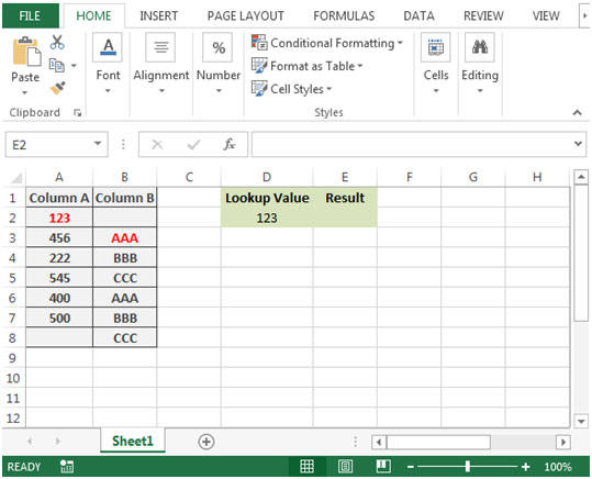
Columns A& B contain numbers and matching letters.However, rather than being adjacent, each letter in column B is shifted down one row with respect to its matching number in column A.We need a formula in cell E2 to lookup the value in cell D2 to find the output.


The applications/code on this site are distributed as is and without warranties or liability. In no event shall the owner of the copyrights, or the authors of the applications/code be liable for any loss of profit, any problems or any damage resulting from the use or evaluation of the applications/code.