If you want to retrieve the column header that corresponds with a matched value,you can use a combination of INDEX, MAX, SUMPRODUCT & COLUMN functions to extract the output.
INDEX: Returns a value or reference of the cell at the intersection of a particular row and column, in a given range.
Syntax: =INDEX(array,row_num,column_num)
MAX: Returns the maximum number from a range of cells or array. For example,if a list of numbers contains 5, 6, 7, 8, 9 & 10, then the output will be 10.
Syntax =MAX(number1,number2,...)
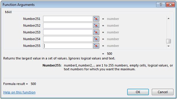
There can be a maximum 255 arguments.Refer below shown screenshot:

SUMPRODUCT: Returns the sum of the products of corresponding ranges or arrays.
Syntax: =SUMPRODUCT(array1,array2,array3,...)
array1,array2,….. array255 are the ranges of cells or arrays that you want to multiply & then add them.
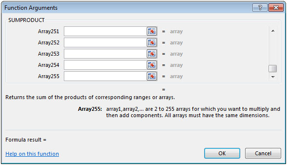
There can be maximum 255 arrays in SUMPRODUCT function.Refer below shown screenshot:

COLUMN: Returns the column number of a reference.
Syntax: =COLUMN(reference)
Let us take an example:
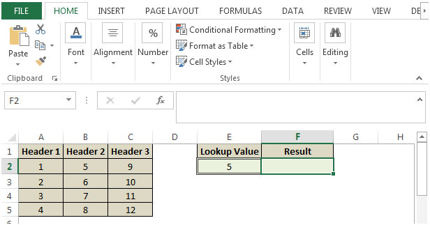
We have 3 column headers that contain numeric values.We need a formula to lookup in cell E2 & retrieve result in cell F2 should be the heading of that column.
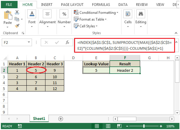
Selecting a value from column B in cell E2 the result should be the column heading in cell F2.

lookup value is 5 refer below snapshot:


The applications/code on this site are distributed as is and without warranties or liability. In no event shall the owner of the copyrights, or the authors of the applications/code be liable for any loss of profit, any problems or any damage resulting from the use or evaluation of the applications/code.
Thank you so much. Very helpful tip.
This formula breaks if any of the cells in the lookup range are blank. How do I get this formula to ignore blank cells in the data range?
What if you have 2 of the same look up numbers can you make the results of both headers?
how do i make it so that the exact value is looked up and column header retrieved? I looked up a value that isn't within the table on purpose and just got the closest value -> column header of that closest value. I would like it to say error to tell me the value i'm looking for doesn't exist.
=iferror(INDEX($A$1:$C$1,SUMPRODUCT(MAX(($A$2:$C$5=E2)*(COLUMN($A$2:$C$5))))-COLUMN($A$1)+1),"")