How to Find the Last Value in a Dynamic List

To retrieve the last value in a dynamic list, wewill use the Data Validation option along with the OFFSET and COUNTA functionsin Microsoft Excel 2010/2013.

COUNTA: It returns the count of the number of cells which contain values.

Syntax of “COUNTA” function: =COUNTA (value1, value2, value3…….)

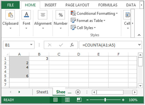
Example: In range A1:A5, cells A2, A3 and A5 contain the values, and cells A1and A4 are blank.  Select the cell A6 and write the formula-

                        =COUNTA(A1:A5) the function will return 3

OFFSET: It returns a reference to a range that is offset a number of rows and columns from another range or cell.

Syntax of OFFSET function:    =OFFSET (reference, rows, cols, height, width)

Reference:- This is the cell or range from which you want to offset.

Rows and Columns to move: - How many rows you want to move the starting point and both of these can be positive, negative or zero.

Height and Width: - This is the size of the range you want to return. This is an optional field.

Let’s take an example to understand the Offset function in Excel.

We have data in range A1:D10. Column A contains Product Code, Column B contains Quantity, column C contains per product cost and column D contains Total cost. We need to return the value of cell C5 in cell E2.

Follow the below mentioned steps.

• Select the cell E2 and write the formula.
• =OFFSET(A1,4,2,1,1)and press Enter on the keyboard.
• The function will return the value of cell C5.

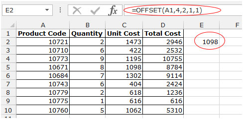
In this example, we need to obtain the value from cell C5 into E2.  Our reference cell is the first cell in the range which is A1 and C5 is 4 rows below and 2 columns to the right from A1.  Hence, the formula is =OFFSET(A1,4,2,1,1) or =OFFSET(A1,4,2) (since 1,1 is optional).

Now, let’s take an example to retrieve the last value in a dynamic list.

We have country names in a range. Now, if we add more countriestothis list, it should be available in the drop down list automatically.

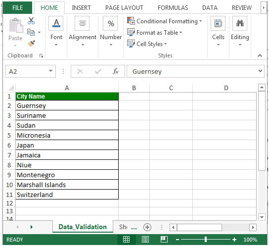
To prepare a dynamic list,we need to create a formula which will retrieve the last value in the column and automatically update when a new number is added.

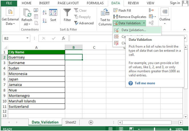
Followthe below given steps:-

• Select the cell B2.
• Go to the Data tab, select Data Validation from the Data tools group.

• The “Data Validation” dialog box will appear. In the “Settings” tab select “Custom” from the Allow drop down list.

• The formula box will be activated.
• Write the formula in this box.
• =OFFSET(A:A,1,0,COUNTA(A:A)-1,1).
• Click on OK.

• At this stage, the last updated cell is A11.

• To check if the Data Validation is working properly, add a city name in cell A12.

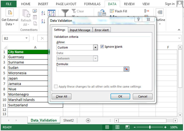
As soon as you add an entry in A12, it will be added to the dropdown list.

This is the way you can create a dynamic list and populate new entries into it automaticallyin Microsoft Excel 2010 and 2013.