Retrieving Values Using References Based on Row and Column Numbers in Microsoft Excel 2010

To retrieve the values using references based on row & column numbers, we will use a combination of "INDIRECT"& "ADDRESS" functions to get the output.
INDIRECT: Returns the reference specified by a text string.

Syntax: =INDIRECT(ref_text,A1)
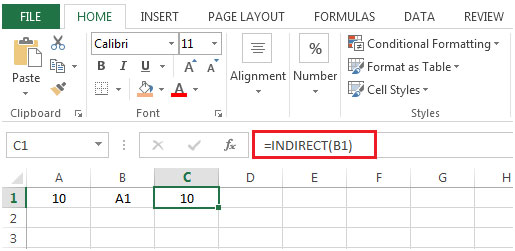
Example: If value in cell A1 contains 10, B1 contains A1 & we use INDIRECT function in cell C1=INDIRECT(B1), then result would be 10

ADDRESS: Creates a cell reference as text, given specified row & column numbers

Syntax: =ADDRESS(row_num,column_num,abs_num,A1,sheet_text)

Let us take an example:

Column A & B contain some random numbers. We need a formula to look for row number & column number & then find the value of that cell.

• In above shown example, if row is selected as 3 & column as 2 then we are looking after value of cell B3.
• The formula in cell F2 would be
• =INDIRECT(ADDRESS(D2,E2))
• Press enter on your keyboard.
• The function will return the value which is in 3^rd row and 2^nd column.