Returning the Entire Contents of the Row Containing the Highest Math Grade

In this article we will learn how to return the entire content of the row containing the highest math grade in Microsoft Excel 2010.

If you want to find the entire contents of the row containing the highest Math Grade, you can use a combination of INDEX, MATCH & MAX functions to extract the output.
INDEX: Returns a value or reference of the cell at the intersection of a particular row and column, in a given range.

Syntax: =INDEX(array,row_num,column_num)
MATCH function searches for a specified item in a selected range of cells, and then returns the relative position of that item in the range.

Syntax =MATCH(lookup_value,lookup_array,match_type)
MAX: Returns the maximum number from a range of cells or array. For example, if a list of numbers contains 5, 6, 7, 8, 9 & 10, then the output will be 10.

Syntax =MAX(number1,number2,...)

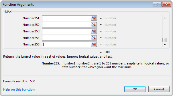
There can be maximum 255 arguments. Refer below shown screenshot:

Let us take an example:

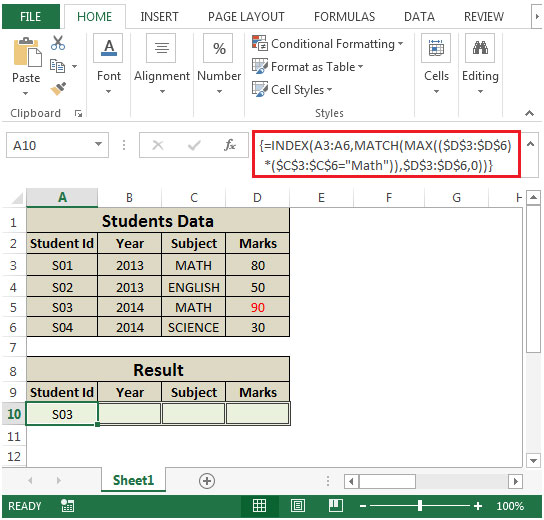
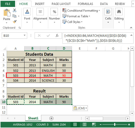
We have Students Data as Student ID in column A, Year in column B, Subject in column C & Marks in column D respectively. We need a formula in range A10:D10 to retrieve the entire contents of the row based on the highest marks for Mathematics subject.

In cell A10, the formula would be
=INDEX(A3:A6,MATCH(MAX(($D$3:$D$6)*($C$3:$C$6="Math")),$D$3:$D$6,0))
Press CTRL + SHIFT + ENTER, this is an array formula.
Formula will be look like this:- {=INDEX(A3:A6,MATCH(MAX(($D$3:$D$6)*($C$3:$C$6="Math")),$D$3:$D$6,0))}

By copying the formula from cell A10 to range B10:D10, we will get the desired result.

The function will return the entire content of the row containing the highest Math grade.

Mo-Alaa
March 20, 2019 at 1:37 pm

I have a case similar to this case as i have a groub of customers and i want to have the data of last transaction for each one ( Date, receipt number, paid amount and the (product or reason) ).
I think this abroach Explaind in your topic is similar to what i'm looking for.

Reply ↓
- Exceltip
  August 10, 2019 at 12:08 pm
  
  So, if you have date in A2:A6, reciept in B2:B6 and paid amount in C2:C6 then write these formulas to get last transaction data
  for Date
  =INDEX(A2:A6,MATCH(MAX(A2:A6),A2:A6,0))
  for Reciept
  =INDEX(B2:B6,MATCH(MAX(A2:A6),A2:A6,0))
  for paid amount,
  =INDEX(C2:C6,MATCH(MAX(A2:A6),A2:A6,0)).
  
  It's a normal formula that gets the index of latest date and then uses that index retrieves all different columns.
  
  Reply ↓