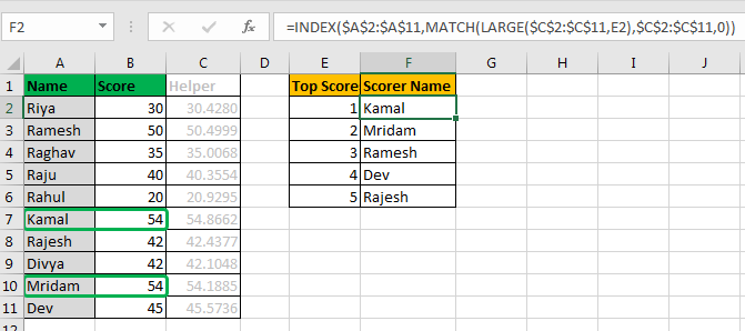
In this article, we will learn how to lookup for multiple value with duplicate lookup values in Excel.

So here is the scenario. I have 10 students. I prepared an exam. In that exam each student scored marks out of 100. Now in Excel, i want to write a formula that tells me top 5 scorer’s name.

Apparently I can use the LARGE function, to get top values. And then VLOOKUP-CHOOSE or INDEX-MATCH function to trace down the names.
But the problem here is that it has clashing scores. And when you try to use INDEX-MATCH, it will return the first name found for same scores. It will not fetch the second name of duplicate score.

You can see that we have two top scorers, Kamal and Mridam who scored 54. But only kamal’s name is fetched on both positions.
This formula is fine, it just need a little help to identify each score uniquely. So we need a helping column here.
In C2, write this formula and copy through C11.

The RAND function returns a random number between 1 and 0.
Now this column adds a random number to scores. Since the added number is between 1 and 0, there will be no significant change to actual score.
Now we can use this column to get our top 4 scorer’s names.
Here
LARGE($C$2:$C$11,E2): LARGE function in Excel will return the nth Largest number from range $C$2:$C$11, which will be a unique value.
MATCH(LARGE($C$2:$C$11,E2),$C$2:$C$11,0): Match function will look for that max value in range $C$2:$C$11, and will return it’s index.
INDEX($A$2:$A$11,MATCH(LARGE($C$2:$C$11,E2),$C$2:$C$11,0)): Now INDEX function will look at that index in range $A$2:$A$11, and will return name at that Position.
You can hide this Helper column or make it invisible using colours.
Note that it works only for numeric values. It will fail for text values. If you want to VLOOKUP Multiple Values with duplicate lookup values then it will not work.
I hope this was helpful. Let me know if you have any specific requirement. Write it in the comments section below.
Related Articles:
How to VLOOKUP Multiple Values in Excel
How to use the INDEX and MATCH to Lookup Value in Excel
How to Lookup Value with Multiple Criteria in Excel
Popular Articles:
50 Excel Shortcuts to Increase Your Productivity
How to use the VLOOKUP Function in Excel
The applications/code on this site are distributed as is and without warranties or liability. In no event shall the owner of the copyrights, or the authors of the applications/code be liable for any loss of profit, any problems or any damage resulting from the use or evaluation of the applications/code.
Hello,
I am in need of some assistance with the following data set:
A B C
0 1.096910013 0
0 1.397940009
4.08 1.698970004
4.95 2
8.09 2.301029996
8.09 2.602059991
8.09 2.903089987
I need Excel to return the max value associated with 0 (cell C2); cell C2 will change for each dataset so I need the formula to include that as the reference so it works every time. It's rare that future data sets will include multiple zeros, so I'd like to make the formula where it will still work when I don't have duplicates (i.e. still return the value associated with value in cell C2).
Any help you can provide is greatly appreciated!