In this article, we will learn about how to use the MROUND function in Excel.
Syntax:
Number : around the number
Multiple : resulting number multiple of a number
The MROUND function returns a multiple of the given value (multiple) nearest to the number. Unlike ROUND function which just rounds off the number.
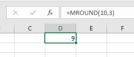
For example: =MROUND(10,3) returns 9

The functions finds the closest number to the 10 which is a multiple of 3.
Let’s understand this function using it an example.

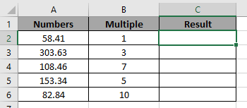
Here we have some numbers and its Multiple.
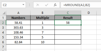
We need to find the multiple of 1 which is closest to 58.41.
Use the Formula:
A2 : number
B2 : multiple

We knew 58 will be the closest number to 58.41 which is multiple of 1.
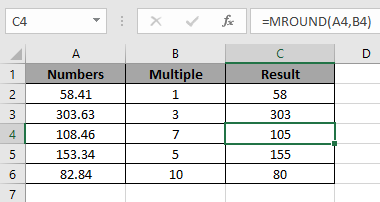
Now copy the formula in the cell using shortcut key Ctrl + D.

As you can see the function returns the multiple of the numbers
Hope you understood how to use MROUND function in Excel. Explore more articles on Excel ROUND function here. Please feel free to state your query or feedback for the above article.
Related Articles:
Formula Round to nearest 100 and 1000
How to Use Round function in Excel
How to Use RoundUp function in Excel
How to Use Rounddown function in Excel
Rounding Numerical Calculation Results In Microsoft Excel
Popular Articles:
How to use the VLOOKUP Function in Excel
The applications/code on this site are distributed as is and without warranties or liability. In no event shall the owner of the copyrights, or the authors of the applications/code be liable for any loss of profit, any problems or any damage resulting from the use or evaluation of the applications/code.