In this article, we will learn about how to use the OCT2HEX function in Excel.
OCT2HEX function in excel is used to convert octal representation of numbers of radix 8 to hexadecimal numbers (radix = 2).
The table shown below shows you some of the most used base & their radix of Alpha - numeric characters
| Base | radix | Alpha-Numeric Characters |
| binary | 2 | 0 - 1 |
| Octal | 8 | 0 - 7 |
| Decimal | 10 | 0 - 9 |
| hexadecimal | 16 | 0 - 9 & A - F |
| hexatridecimal | 36 | 0 - 9 & A - Z |
octal number representation have 8 digits from 0, 1, 2, 3, 4, 5, 6, 7 and where hexadecimal number is representation of a number of radix 16. 10 digits starting from 0, 1, 2, 3, 4, 5, 6, 7, 8 ,9 along with 6 alphabets starting from A, B, C, D, E & F. The below table will help you understand better.
| Octal | Decimal | hexadecimal |
| 0 | 0 | 0 |
| 1 | 1 | 1 |
| 2 | 2 | 2 |
| 3 | 3 | 3 |
| 4 | 4 | 4 |
| 5 | 5 | 5 |
| 6 | 6 | 6 |
| 7 | 7 | 7 |
| 10 | 8 | 8 |
| 11 | 9 | 9 |
| 12 | 10 | A |
| 13 | 11 | B |
| 14 | 12 | C |
| 15 | 13 | D |
| 16 | 14 | E |
| 17 | 15 | F |
Conversion formulation is in two steps. First the number be converted to binary and then binary number is converted to get the hexadecimal value.
Let’s take an example
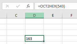
543 is converted to binary number
| 5 | 4 | 3 |
| 101 | 100 | 11 |
| 101 | 100 | 011 |
| 543 ( octal ) = 101 100 011( binary) | ||
101100011 is converted to hexadecimal
| 101100011 | ||
| 0001 | 0110 | 0011 |
| 1 | 6 | 3 |
| 543 ( octal ) = 163 ( hexadecimal) | ||
The OCT2HEX function converts the octal number of radix 8 to the hexadecimal number of radix 2.
Syntax:
Number : Octal number which returns the 10 character hexadecimal number.
[Places] : [optional] number where result expressed upto the number.
The input value to the function cannot contain more than 10 characters ( 10 bits ). Where first number returns the sign of the number (positive or negative) & Other 9 returns the value after the sign. ( 1 for negative & 0 for positive).

To get a negative number, input number must have 10 characters starting with 1 as it represents the negative sign. The negative number is calculated using two's complement notation. Any less than 10 characters, the function considers default 0s in front. Any more than 10 characters, the function returns the #NUM! Error.
Now let’s get more understanding of the function via using them in some examples.

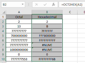
Here we have some octal values in Octal Column. We need to convert these octal numbers to hexadecimal value.
Use the formula in octal column:
A2 : number provided to the function as cell reference
Values to the OCT2HEX function is provided as cell reference.

The OCT2HEX representation of 2 of base 8 (hexadecimal) is 10 of base 2 (decimal).
Now copy the formula to other cells using the Ctrl + D shortcut key.

As you can see here the OCT2HEX function returns the result of the input values.
Notes:
Hope you understood how to use OCT2HEX function and referring cell in Excel. Explore more articles on Excel mathematical conversion functions here. Please feel free to state your query or feedback for the above article.
Related Articles:
How to use the DEC2BIN Function in Excel
How to use the BIN2OCT Function in Excel
How to use the BIN2HEX Function in Excel
How to use the DEC2OCT Function in Excel
How to use the DEC2HEX Function in Excel
How to use the OCT2BIN Function in Excel
How to use the OCT2DEC Function in Excel
How to use the OCT2HEX Function in Excel
How to use the HEX2BIN Function in Excel
How to use the HEX2OCT Function in Excel
How to use the HEX2DEC Function in Excel
Popular Articles:
The applications/code on this site are distributed as is and without warranties or liability. In no event shall the owner of the copyrights, or the authors of the applications/code be liable for any loss of profit, any problems or any damage resulting from the use or evaluation of the applications/code.