In this article, we will learn about how to use the PERCENTRANK function in Excel.
The PERCENTRANK is a statistical function. In statistics, finding a percentage or percentile for the number on an array of numbers.
The function checks the place of value on the list of values and returns its percentage place on the list of values.
PERCENTRANK function takes the range of values as array and value. And returns the interpolate percentile for the given value.
Syntax:
| =PERCENTRANK (array, x, [significance]) |
array : a list of numbers
x : number or value
[significance] : value upto decimal places. Default is 3.
Example:
Let’s understand this function using it as an example.
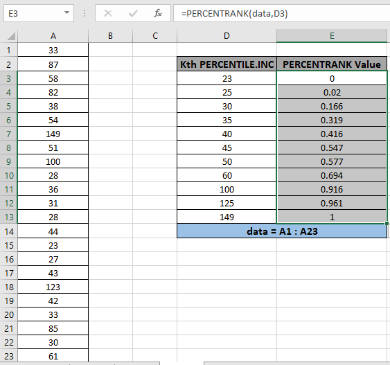
Here we have a set of values as data ( A1 : A23 ) and we need to find some PERCENTRANK values for the values. [significance] is set to default which is 3.

Use the formula:
| = PERCENTRANK ( data , D3) |
data - array given using named range.
D3 - value to which percentile is calculated.

The function returns the percentage for the value ( 23 ) PERCENTRANK value or minimum value for which the percentile is 0 .
Now copy the formula to get different PERCENTRANK values of the range to the remaining cells and formula as shown in the snapshot below.

As you can see the results in the snapshot above.
Here are some of the observations gathered using the PERCENTRANK function.
Note:
Hope you understood How to use the PERCENTRANK function in Excel. Explore more articles on statistical functions like SMALL function & LARGE function here. Please state your query in the comment box below.
Related Articles
How to use the QUARTILE function in Excel
How to use the LARGE function in Excel
How to use the SMALL function in Excel
Popular Articles
The applications/code on this site are distributed as is and without warranties or liability. In no event shall the owner of the copyrights, or the authors of the applications/code be liable for any loss of profit, any problems or any damage resulting from the use or evaluation of the applications/code.