Find the Last Value in Column in Microsoft Excel

In this article, we will learn how to find the last numeric value in a range. We can use the “Index” function along with “Match” function in Microsoft Excel 2010 to get the desired output.

MATCH: Match formula returns the cell number where the value is found in a horizontal or vertical range.

Syntax of “MATCH” function:=MATCH(lookup_value,lookup_array,[match_type])

There are 3 match types. 1^st is 1-less than, 2^nd is 0-Exact match, 3^rd is (-1)-greater than.

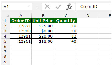
For example:- We have data in range A1:C5 in which column A contains Order Id, column B contains Unit Price, and column C contains Quantity.

To get the last value in column follow below given steps:-

• Write the formula in cell D2.
• =MATCH(12982,A2:A5,1)
• Press Enter on your keyboard.
• The function will return 4, which means 4^th cell is matching as per given criteria.

INDEX: The Index formula returns a value from the intersection between the row number and the column number in an Array. There are 2 syntaxes for the “INDEX” function.

1st Syntax of “INDEX” function:
=INDEX (array, row_num, [column_num])

2nd Syntax of “INDEX” function:
=INDEX (reference, row_num, [column_num], [area_num])

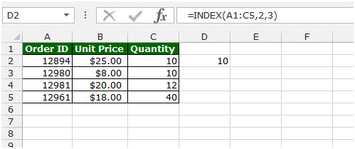
For example: - We have data in range A1:C5 in which column A contains Order Id, column B contains Unit Price, and column C contains Quantity.

Follow below given steps:-

• Write the formula in cell D2.
• =INDEX(A1:C5,2,3)
• Press Enter on your keyboard.
• The function will return 10, which means 10 is available in 2^nd row and 3^rd column.

Let’s take an example to understand how we can find the last numeric value in a range in Microsoft Excel.

We have a list in column A in which some cells contain text and some cells carry values.

If we want to find the last numeric value in the range, then we need to follow below given steps:-

• Write the formula in cell B2.
• =INDEX(A1:A6,MATCH(9.99999999999999E+307,A1:A6))
• Press Ctrl+Shift+Enter on your keyboard.
• After pressing the Ctrl+Shift+Enter, formula will look like this:-
• {=INDEX(A1:A6,MATCH(9.99999999999999E+307,A1:A6))}.
• The function will return 8956, which means this number is the last numeric value in the range.

This is the how we can find the last numeric value in a range by using the Index function along with Match function in Microsoft Excel.