
If you want to sum up the 3 values in Excel you can do it by simply calculating the top 3 values using a LARGE function and sum them up.
But that's not the only way. You can sum top N values in Excel using multiple formulas. All of them will use the LARGE function as the key function. See the image above. Let's explore them all.
Generic formula
| =SUMIF(range,">="&LARGE(range,n)) |
Range: The range is the range from which you want to sum top N values.
n: This is the number of top values that you want to sum up. If you want to sum top 3 values then n is 3.
So let's see this formula in action.
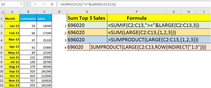
We have data that contains the sales done in different months. We need to sum up the top 3 sales. We use the generic formula above.
The range is C2:C13 and n is 3. Then the formula will be:
| =SUMIF(C2:C13,">="&LARGE(C2:C13,3)) |
This returns to 696020 which is correct. If you want to sum up top variable N values and N is written in D2 then the formula will be:
| =SUMIF(C2:C13,">="&LARGE(C2:C13,D2)) |
it will sum up all the values that are greater than or equal to the value of the top N value.
The LARGE function returns the top Nth value in the given range. In the formula above, the LARGE function returns the third largest value in range C2:C13 which is 212940. Now the formula is:
| =SUMIF(C2:C13,">="&212940) |
Now the SUMIF function simply returns the SUM of values greater than or equal to 212940, which is 696020.
If you want to add multiple conditions to sum top 3 or N values, use SUMIFS function.
The above method is quite easy and fast to use when it comes to sum up the top 3 or N values from the list. But it gets difficult when it comes to summing top arbitrary N values, say top 2nd, 4th, and 6th value from an Excel range. Here, the SUM or SUMPRODUCT function gets the work done.
Generic Formula:
| =SUM(LARGE(range,{1,2,3})) |
or
| =SUMPRODUCT(LARGE(range,{1,2,3})) |
Range: The range is the range from which you want to sum up top N values.
{1,2,3}: These are the top values that you want to sum up. Here it is 1st, 2nd, and 3rd.
So let's use this formula in the example above.
So, we are using the same table that we used in the example above. The range is still C2:C13 and the top 3 values that we want to sum are 1st, 2nd and 3rd largest values in the range.
| =SUMPRODUCT(LARGE(C2:C13,{1,2,3})) |
It returns the same result as before, which is 696020. If you want to sum up the 2nd and 4th topmost values then the formula will be:
| =SUMPRODUCT(LARGE(C2:C13,{2,4})) |
And the result will be 425360.
You can replace the SUMPRODUCT function with the SUM function in the above case. But if you want to give reference to top values then you will need to use CTRL+SHIF+ENTER to make it an array formula.
| {=SUM(LARGE(C2:C13,E2:E4))} |
How does it work?
The LARGE function accepts an array of key values and returns an array of those top values. Here the large function returns the values {241540;183820;38740} as top 2nd, 4th, and 6th values. Now the formula becomes:
| =SUM({241540;183820;38740}) |
or
| =SUMPRODUCT({241540;183820;38740}) |
This sums up the values returned by the LARGE function.
Let's say you want to sum values top 10-2o values, all-inclusive. In this case, the above-mentioned methods will get fussy and longer. The best way is to use the below generic formula to sum up the top values:
| =SUMPRODUCT(LARGE(range,ROW(INDIRECT("start:end")))) |
range: The range is the range from which you want to sum top N values.
"start:end": It is the text of the range of top values that you want to sum up. If you want some top 3 to top 6 values then start:end will be "3:6".
Let's look at this formula in action:
Example 3: Sum the top 3 to 6 values from sales:
So we have the same table as the above example. The only query is different. Using the above generic formula, we write this formula:
| =SUMPRODUCT(LARGE(C2:C13,ROW(INDIRECT("3:6")))) |
This returns the value 534040. Which is the sum of 3rd, 4th, 5th, and 6th largest value from range C2:C13.
How does this work?
First, the INDIRECT function turns text "3:6" into actual range 3:6. Onwards, ROW function returns an array of row numbers in range 3:6, which will be {3,4,5,6}. Next, the LARGE function returns the 3rd, 4th, 5th, and 6th largest values from the range C2:C13. Finally, the SUMPRODUCT function sums up these values and we get our result.
| =SUMPRODUCT(LARGE(C2:C13,ROW(INDIRECT("3:6"))))
=SUMPRODUCT(LARGE(C2:C13,{3,4,5,6})) =SUMPRODUCT({212940;183820;98540;38740}) = 534040 |
The SEQUENCE function is introduced in Excel 2019 and 365. It returns a sequence of numbers. We can use it to get the top N values and then sum them up.
Generic Formula:
| =SUMPRODUCT(LARGE(range,SEQUENCE(num_values,,[start_num], [steps])))) |
range: The range is the range from which you want to sum top N values.
num_values: It is the number of top values that you want to sum.
[start_num]: It is the starting number of the series. It is optional. If you omit this, the series will start from 1.
[steps]: It is the difference between the next number from the current number. By default, it is 1.
If we use this generic formula to get the same result as we did in the previous example, the formula will be:
| =SUM(LARGE(C2:C13,SEQUENCE(4,,3))) |
It will return the value 534040.
How does it work?
It is simple. The SEQUENCE function returns a series of 4 values that start with 3 with interval 1. It returns the array {3;4;5;6}. Now LARGE function returns the largest values of corresponding numbers. Finally, the SUM function sums up these value and we get our result as 534040.
| =SUM(LARGE(C2:C13,SEQUENCE(4,,3)))
=SUM(LARGE(C2:C13,{3;4;5;6})) =SUM({212940;183820;98540;38740}) =534040 |
So yeah guys, this is how you can sum up the top 3, 5, 10, ... N values in Excel. I tried to be explanatory. I hope it helps you. If you have any doubts regarding this topic or any other excel VBA related topic, ask in the comments section below. I reply to queries frequently.
Related Articles:
Sum If Greater Than 0 in Excel | To sum only positive values, we need to sum values that are greater than 0. To do so, we will use SUMIF function of Excel.
How to Sum Last 30 Days Sales in Excel | Some times it is also summarized on standard 30 day interval. In that case, having a formula that dynamically shows the sum of the last 30 days will be a good idea. In this article, we will learn how to sum the last 30 days' values in excel.
How to sum last n columns in Excel | Sometimes given a condition i.e. when we need to get the sum of the last 5 or n numbers from the column. You can perform the solution to this problem easily using the excel functions.
How to Sum by Matching Row and Column in Excel | How do we sum values when we need to match column and row. In this article, we will learn how to do the sum of matching rows and columns.
Popular Articles:
50 Excel Shortcuts to Increase Your Productivity | Get faster at your task. These 50 shortcuts will make you work even faster on Excel.
How to use Excel VLOOKUP Function| This is one of the most used and popular functions of excel that is used to lookup value from different ranges and sheets.
How to use the Excel COUNTIF Function| Count values with conditions using this amazing function. You don't need to filter your data to count specific value. Countif function is essential to prepare your dashboard.
How to Use SUMIF Function in Excel | This is another dashboard essential function. This helps you sum up values on specific conditions.
The applications/code on this site are distributed as is and without warranties or liability. In no event shall the owner of the copyrights, or the authors of the applications/code be liable for any loss of profit, any problems or any damage resulting from the use or evaluation of the applications/code.


