Summing Annual Expenses by Respective Quarters

If you want a formula that will give you total of the expenses incurred in a quarter based on the value in the corresponding cell.

You can use a combination of SUM, ROUNDUP & MONTH functions to get the output.

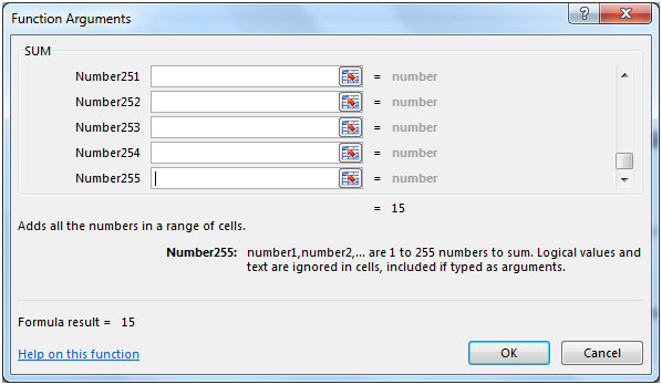
SUM: Adds all the numbers in a range of cells

Syntax: =SUM(number1,number2,...)

There can be maximum 255 arguments. Refer below mentioned screenshot:

MONTH: This function returns the month (January to December as 1 to 12) of a date.

Syntax: =MONTH(serial_number)

ROUNDUP: Rounds a number up, away from zero

Syntax: =ROUNDUP(number,num_digits)

Let us take an example:

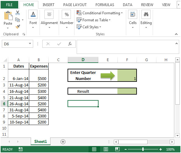
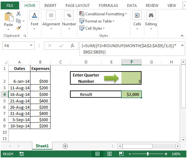
We have Dates in column A & Expenses in column B. We want a formula that will return the sum of the total annual expenses for the particular Quarter of the year. In cell F2, Quarter of the year is entered.

The formula in cell F4 would be
=SUM((F2=ROUNDUP(MONTH($A$2:$A$9)/3,0))*$B$2:$B$9)
Press CTRL + SHIFT + ENTER, because this is an array function.
{=SUM((F2=ROUNDUP(MONTH($A$2:$A$9)/3,0))*$B$2:$B$9)}

We will get the desired result as $ 500 because there is only one date from first quarter.
If we change the quarter number in cell F2, say change to 3, then result would be the sum of the total based on value of the respective quarter.