How to Sum Groups of Every N Values in a Row in Excel

In this article, we will learn How to Sum Groups of Every N Values in a Row in Excel.

Scenario:

For Instance, you have a large list of data and you need to find the SUM of the numbers having a set of n values .

For this article we will be needing the use the following functions:

1. SUM Function
2. OFFSET function

Sum Groups of Every N Values formula in Excel

Now we will make a formula out of these functions. Here we will be given the data and we needed to find the SUM having a specified number of cells.

Formula

explained

• OFFSET function starts from the reference and traverse ro number of rows and co number of columns from the cell reference.
• Now the function starts picking groups of numbers having the number of values in the column and the number of values in the row.
• The OFFSET function now returns the array of numbers to the SUM function.
• SUM function adds up all the numbers and returns the SUM.

Example :

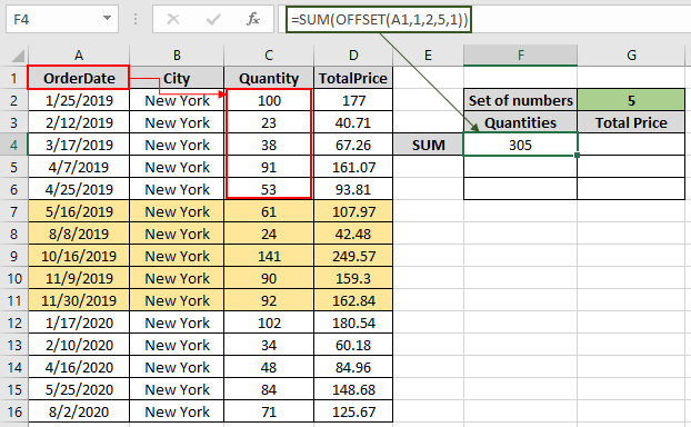
All of these might be confusing to understand. Let's understand how to use the function using an example. Here we have a data from A1 : D16. we need to find the SUM of Quantity & Total Price in a group of 5 with the given reference from the A1 cell.

First we need to find the SUM of first 5 quantity which are values { 100 , 23 , 38 , 91 , 53 }

Use the Formula:

Explanation:

• OFFSET function starts from the A1 cell and reaches the C2 cell traversing the 1 row and 2 columns.
• We need first 5 cells from C2 to C6 cell. So the height 5 and width will return us the numbers as shown below.

= SUM ( { 100 ; 23 ; 38 ; 91 ; 53 } )

• Now the SUM function returns the SUM of the values.

Here the A1 is given as cell reference & rest of the arguments are provided directly to the function.

As you can see in the above snapshot the SUM of first five quantity comes out to be 305 .

Now we will get the SUM for all the other groups of 5 by changing the Row argument of the function

Use the Formula:

As you can see the SUM of next five in the snapshot above. For the next five change the row argument to 11.

Get the SUM of TotalPrice for the same by changing the Column argument to the function.

As you can see from the above formula that you can get the SUM values by groups using the OFFSET function.

Here are all the observational notes using the formula in Excel
Notes :

1. The function returns #VALUE! error if the argument to the function is non-numeric.
2. The formula only works with numbers.
3. The argument array must be of the same length else the function.

Hope this article about How to Sum Groups of Every N Values in a Row in Excel is explanatory. Find more articles on calculating values and related Excel formulas here. If you liked our blogs, share it with your friends on Facebook. And also you can follow us on Twitter and Facebook. We would love to hear from you, do let us know how we can improve, complement or innovate our work and make it better for you. Write to us at info@exceltip.com.

Related Articles :

Sum by OFFSET groups in Rows and Columns : The OFFSET function can be used to sum group of cells dynamically. These groups can be anywhere in the sheet.

SUM if date is between : Returns the SUM of values between given dates or period in excel.

Sum if date is greater than given date: Returns the SUM of values after the given date or period in excel.

2 Ways to Sum by Month in Excel: Returns the SUM of values within a given specific month in excel.

How to Sum Multiple Columns with Condition: Returns the SUM of values across multiple columns having condition in excel

Use INDEX and MATCH to Lookup Value : The INDEX-MATCH formula is used to lookup dynamically and precisely a value in a given table.  This is an alternative to the VLOOKUP function and it overcomes the shortcomings of the VLOOKUP function.

How to use wildcards in excel : Count cells matching phrases using the wildcards in excel.

Popular Articles :

How to use the IF Function in Excel : The IF statement in Excel checks the condition and returns a specific value if the condition is TRUE or returns another specific value if FALSE.

How to use the VLOOKUP Function in Excel : This is one of the most used and popular functions of excel that is used to lookup value from different ranges and sheets.

How to use the SUMIF Function in Excel : This is another dashboard essential function. This helps you sum up values on specific conditions.

How to use the COUNTIF Function in Excel : Count values with conditions using this amazing function. You don't need to filter your data to count specific values. Countif function is essential to prepare your dashboard.