Summing the Visible Filtered List in Excel 2010

To get the total of the values in the visible filtered rows only, we can use the SUBTOTAL function to retrieve the output.
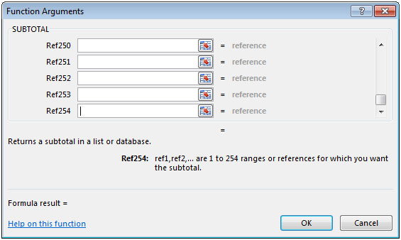
SUBTOTAL:Returns a subtotal in a list or database.

Syntax: =SUBTOTAL(function_num,ref1,...)

Let us take an example:

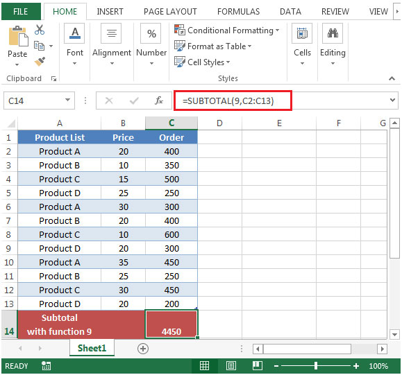
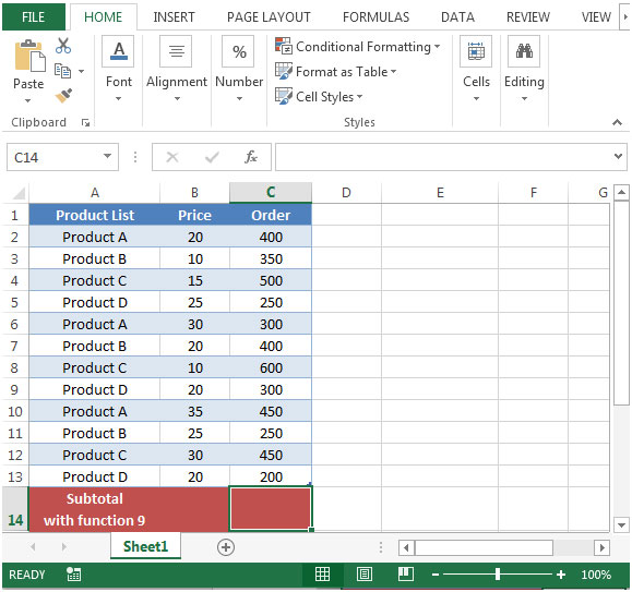
We have Product list in column A, Price in column B & Order in column C.

• In cell C14, the formula would be =SUBTOTAL(9,C2:C13)

• If we apply filter the list with Orders more than 300, the subtotal function will give the sum of the Order which are more than 300.
• Select any cell in table & press CTRL + SHIFT + L for applying Filter.
• Click on Order drop down, select Number Filters.
• Select Greater than option.

• The following dialog box will appear. Enter 300 in the box as shown in screenshot below.

• The table will get filter on the Order list which are more than 300

• You can use SUBTOTAL to ignore values in hidden rows.

We use hide rows to remove unnecessary information from viewer. You can use SUBTOTAL with function as 109 which will ignore the values that are hidden.

• In cell C15, the formula would be =SUBTOTAL(109,C2:C13)& we hide row number 10 where Order value is 450 then the result of SUBTOTAL function will be different when using 109 as first argument.

SUBTOTAL(9,...) totals everything except cells with subtotals and filtered cells.

SUBTOTAL(109,...) totals everything except cells with subtotals and filtered cells and hidden rows.