Sum Formula in Microsoft Excel

In this article we will learn how and where we can use Sum formula in Microsoft Excel.

To add the figures at the intersection of two or more ranges, we can leave a space between the argument ranges in the SUM formula.
SUM: Adds all the numbers in a range of cells

Syntax: =SUM(number1,number2,...)

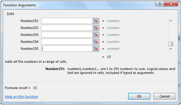
There can be maximum 255 arguments. Refer below shown screenshot:

Let us take an example:

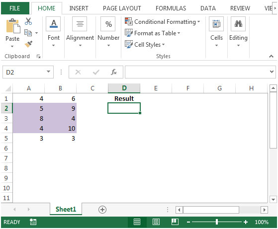
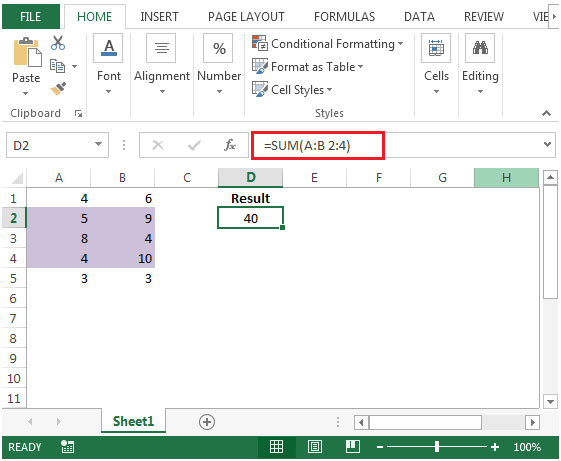
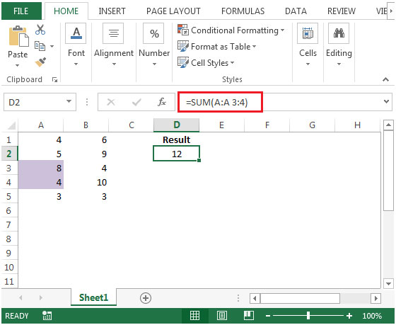
Column A & B contain some random numbers. We need a formula to find the total of specific rows & columns.We will use Sum function along with a space between the argument ranges.We want a total value of the cells occurring at the intersection of the following ranges:

1. Columns A:B, Row 2:4
2. Column A:A, Row 3:4
3. Columns A:B, Row 1:1 + Columns A:B, Row 5:5

To sum only the highlighted portion of the range, the formula would be
=SUM(A:B 2:4)

If we select the range manually, we can see the result in status bar to verify the result.

To get the sum of Column A:A, Row 3:4
In cell D2, the formula would be
=SUM(A:A 3:4)

To Sum Columns A:B, Row 1:1 + Columns A:B, Row 5:5
In cell D2, the formula would be
=SUM(A:B 1:1,5:5)

If you liked our blogs, share it with your friends on Facebook. And also you can follow us on Twitter and Facebook.
We would love to hear from you, do let us know how we can improve, complement or innovate our work and make it better for you. Write us at info@exceltip.com

EEM
May 11, 2015 at 1:56 pm

The following statements are incorrect:
•To Sum Columns A:B, Row 1:1 + Columns A:B, Row 5:5
•In cell D2, the formula would be
=SUM(A:B 1:1,5:5)

As the formula =SUM(A:B 1:1,5:5) includes the entire row 5 not just columns A and B, the result shown is correct because only columns A and B contain values.

The correct formula would be:
=SUM(A:B 1:1,A:B 5:5)
Or
=SUM(A1:B1,A5:B15) find this practical

Reply ↓